Chapter 3 From verbal to formal models
3.1 Learning Objectives
By the end of this exercise, you will be able to:
- Transform verbal descriptions of decision-making strategies into formal computational models
- Implement and test different agent-based models in R
- Compare and evaluate the performance of different strategic agents
- Visualize and interpret simulation results at scale
By computationally implementing the our models,
we are forced to make them very explicit in their assumptions;
we become able to simulate the models in a variety of different situations and therefore better understand their implications
So, the steps for today’s exercise are:
choose two of the models and formalize them, that is, produce an algorithm that enacts the strategy, so we can simulate them.
implement the algorithms as functions: getting an input and producing an output, so we can more easily implement them across various contexts (e.g. varying amount of trials, input, etc). See R4DataScience, if you need a refresher: https://r4ds.had.co.nz/functions.html
implement a Random Bias agent (choosing “head” 70% of the times) and get your agents to play against it for 120 trials (and save the data)
implement a Win-Stay-Lose-Shift agent (keeping the same choice if it won, changing it if it lost) and do the same.
Now scale up the simulation: have 100 agents for each of your strategy playing against both Random Bias and Win-Stay-Lose-Shift and save their data.
Figure out a good way to visualize the data to assess which strategy performs better, whether that changes over time and generally explore what the agents are doing.
3.3 Implementing a random agent
Remember a random agent is an agent that picks at random between “right” and “left” independently on what the opponent is doing. A random agent might be perfectly random (50% chance of choosing “right”, same for “left”) or biased. The variable “rate” determines the rate of choosing “right”.
rate <- 0.5

RandomAgent <- rbinom(trials, 1, rate) # we simply sample randomly from a binomial

# Now let's plot how it's choosing
d1 <- tibble(trial = seq(trials), choice = RandomAgent)

p1 <- ggplot(d1, aes(trial, choice)) +
  geom_line() +
  labs(
    title = "Random Agent Behavior (rate 0.5)",
    x = "Trial Number",
    y = "Choice (0/1)"
  ) +
  theme_classic()
p1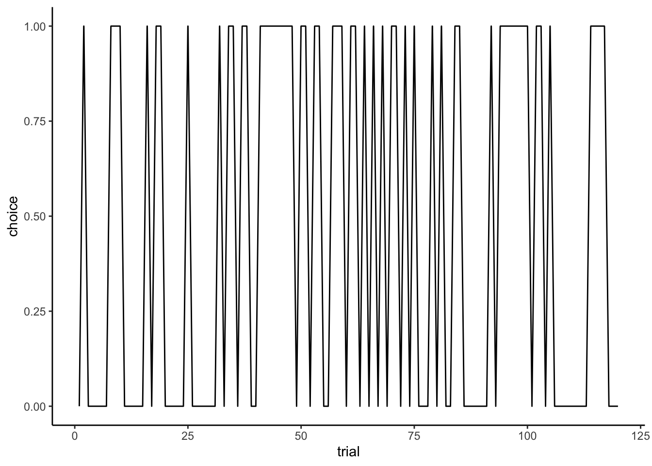
# What if we were to compare it to an agent being biased?
rate <- 0.8

RandomAgent <- rbinom(trials, 1, rate) # we simply sample randomly from a binomial

# Now let's plot how it's choosing
d2 <- tibble(trial = seq(trials), choice = RandomAgent)
p2 <- ggplot(d2, aes(trial, choice)) +
  geom_line() +
  labs(
    title = "Biased Random Agent Behavior",
    x = "Trial Number",
    y = "Choice (0/1)"
  ) +
  theme_classic()

p1 + p2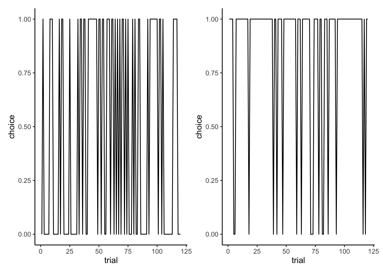
# Tricky to see, let's try writing the cumulative rate:

d1$cumulativerate <- cumsum(d1$choice) / seq_along(d1$choice)
d2$cumulativerate <- cumsum(d2$choice) / seq_along(d2$choice)

p3 <- ggplot(d1, aes(trial, cumulativerate)) +
  geom_line() +
  ylim(0,1) +
  labs(
    title = "Random Agent Behavior",
    x = "Trial Number",
    y = "Cumulative probability of choosing 1 (0-1)"
  ) +
  theme_classic()

p4 <- ggplot(d2, aes(trial, cumulativerate)) +
  geom_line() +
  labs(
    title = "Random Agent Behavior",
    x = "Trial Number",
    y = "Cumulative probability of choosing 1 (0-1)"
  ) +
  ylim(0,1) +
  theme_classic()

p3 + p4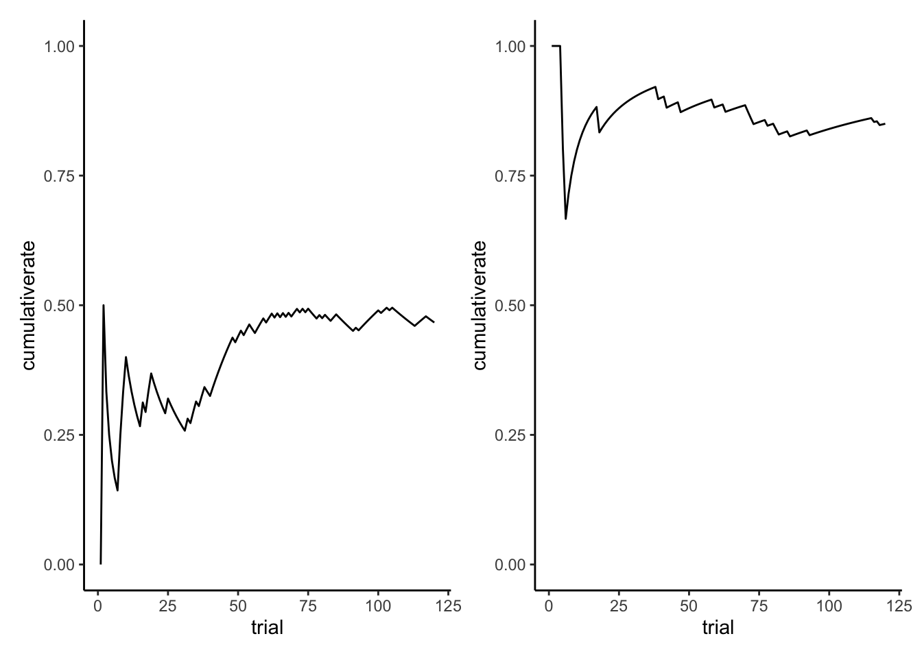
## Now in the same plot
d1$rate <- 0.5
d2$rate <- 0.8
d <- rbind(d1,d2) %>%
  mutate(rate = as.factor(rate))

p5 <- ggplot(d, aes(trial, cumulativerate, color = rate, group = rate)) +
  geom_line() +
  labs(
    title = "Random Agents Behavior",
    x = "Trial Number",
    y = "Cumulative probability of choosing 1 (0-1)"
  ) +
  ylim(0,1) +
  theme_classic()
p5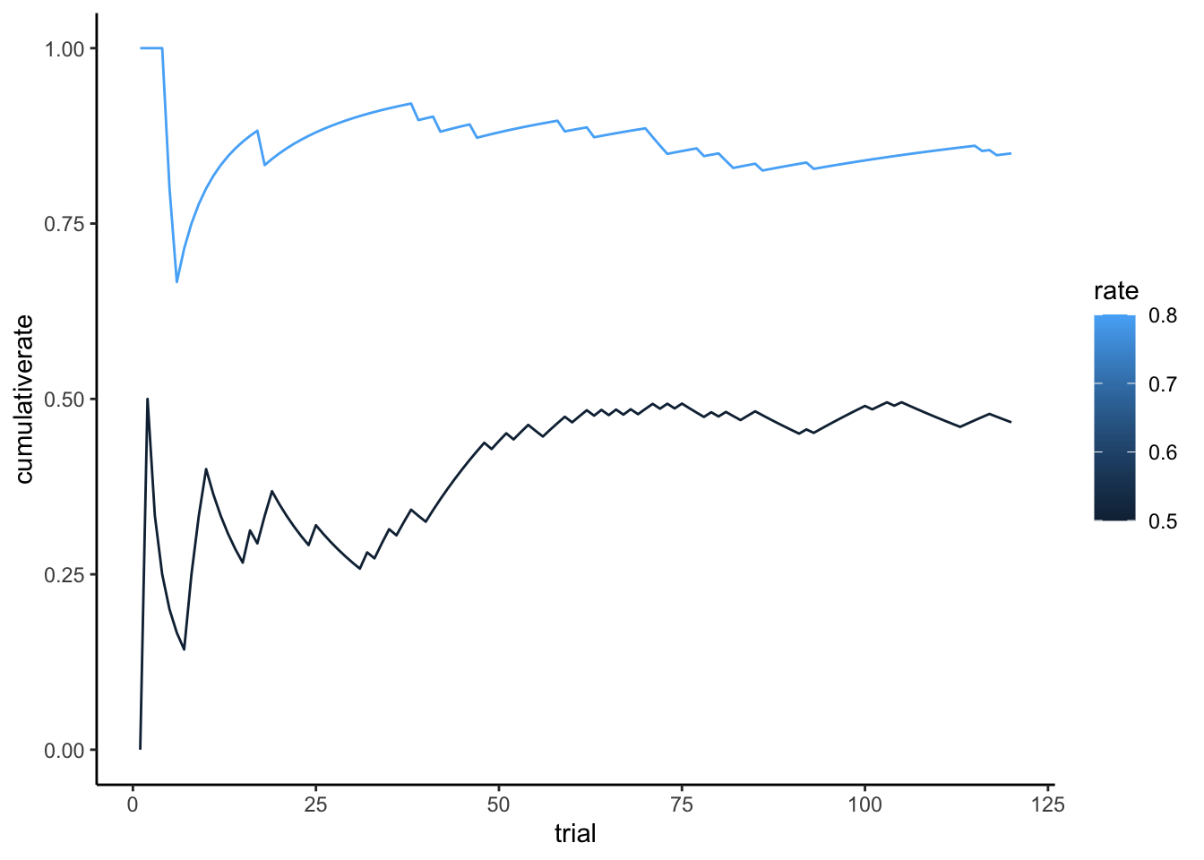
# Now as a function
#' Create a random decision-making agent
#' @param input Vector of previous choices (not used but included for API consistency)
#' @param rate Probability of choosing option 1 (default: 0.5 for unbiased)
#' @return Vector of binary choices
#' @examples
#' # Create unbiased random agent for 10 trials
#' choices <- RandomAgent_f(rep(1,10), 0.5)
RandomAgent_f <- function(input, rate = 0.5) {
  # Input validation
  if (!is.numeric(rate) || rate < 0 || rate > 1) {
    stop("Rate must be a probability between 0 and 1")
  }

  n <- length(input)
  choice <- rbinom(n, 1, rate)
  return(choice)
}

input <- rep(1,trials) # it doesn't matter, it's not taken into account
choice <- RandomAgent_f(input, rate)
d3 <- tibble(trial = seq(trials), choice)

ggplot(d3, aes(trial, choice)) +
  geom_line() +
  labs(
    title = "Random Agent Behavior",
    x = "Trial Number",
    y = "Cumulative probability of choosing 1 (0-1)"
  ) +
  theme_classic()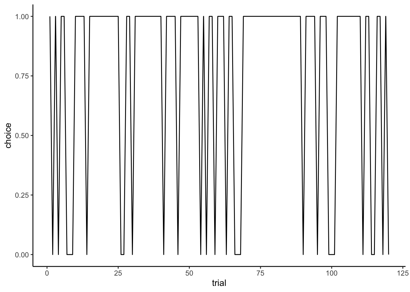
3.4 Implementing a Win-Stay-Lose-Shift agent
#' Create a Win-Stay-Lose-Shift decision-making agent
#' @param prevChoice Previous choice made by the agent (0 or 1)
#' @param feedback Success of previous choice (1 for win, 0 for loss)
#' @param noise Optional probability of random choice (default: 0)
#' @return Next choice (0 or 1)
#' @examples
#' # Basic WSLS decision after a win
#' next_choice <- WSLSAgent_f(prevChoice = 1, feedback = 1)
WSLSAgent_f <- function(prevChoice, feedback, noise = 0) {
  # Input validation
  if (!is.numeric(prevChoice) || !prevChoice %in% c(0,1)) {
    stop("Previous choice must be 0 or 1")
  }
  if (!is.numeric(feedback) || !feedback %in% c(0,1)) {
    stop("Feedback must be 0 or 1")
  }
  if (!is.numeric(noise) || noise < 0 || noise > 1) {
    stop("Noise must be a probability between 0 and 1")
  }

  # Core WSLS logic
  choice <- if (feedback == 1) {
    prevChoice  # Stay with previous choice if won
  } else {
    1 - prevChoice  # Switch to opposite choice if lost
  }

  # Apply noise if specified
  if (noise > 0 && runif(1) < noise) {
    choice <- sample(c(0,1), 1)
  }

  return(choice)
}


WSLSAgentNoise_f <- function(prevChoice, Feedback, noise){
  if (Feedback == 1) {
    choice = prevChoice
  } else if (Feedback == 0) {
      choice = 1 - prevChoice
  }
  if (rbinom(1, 1, noise) == 1) {choice <- rbinom(1, 1, .5)}
  return(choice)
}

WSLSAgent <- WSLSAgent_f(1, 0)


# Against a random agent

Self <- rep(NA, trials)
Other <- rep(NA, trials)

Self[1] <- RandomAgent_f(1, 0.5)
Other <- RandomAgent_f(seq(trials), rate)


for (i in 2:trials) {
  if (Self[i - 1] == Other[i - 1]) {
    Feedback = 1
  } else {Feedback = 0}
  Self[i] <- WSLSAgent_f(Self[i - 1], Feedback)
}

sum(Self == Other)
## [1] 78df <- tibble(Self, Other, trial = seq(trials), Feedback = as.numeric(Self == Other))
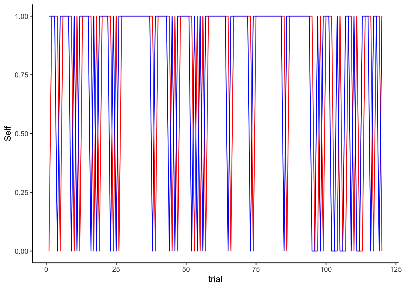
ggplot(df) + theme_classic() +
geom_line(color = "red", aes(trial, Self)) +
geom_line(color = "blue", aes(trial, Other)) +
labs(
title = "WSLS Agent (red) vs Biased Random Opponent (blue)",
x = "Trial Number",
y = "Choice (0/1)",
color = "Agent Type"
)
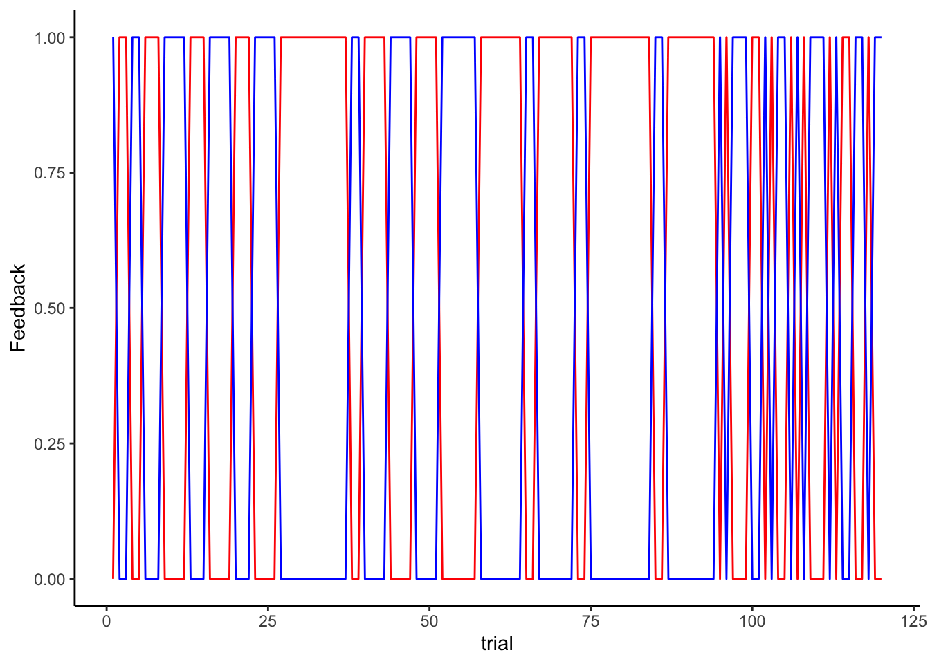
ggplot(df) + theme_classic() +
  geom_line(color = "red", aes(trial, Feedback)) +
  geom_line(color = "blue", aes(trial, 1 - Feedback)) +
  labs(
    title = "WSLS Agent (red) vs Biased Random Opponent (blue)",
    x = "Trial Number",
    y = "Feedback received (0/1)",
    color = "Agent Type"
  )
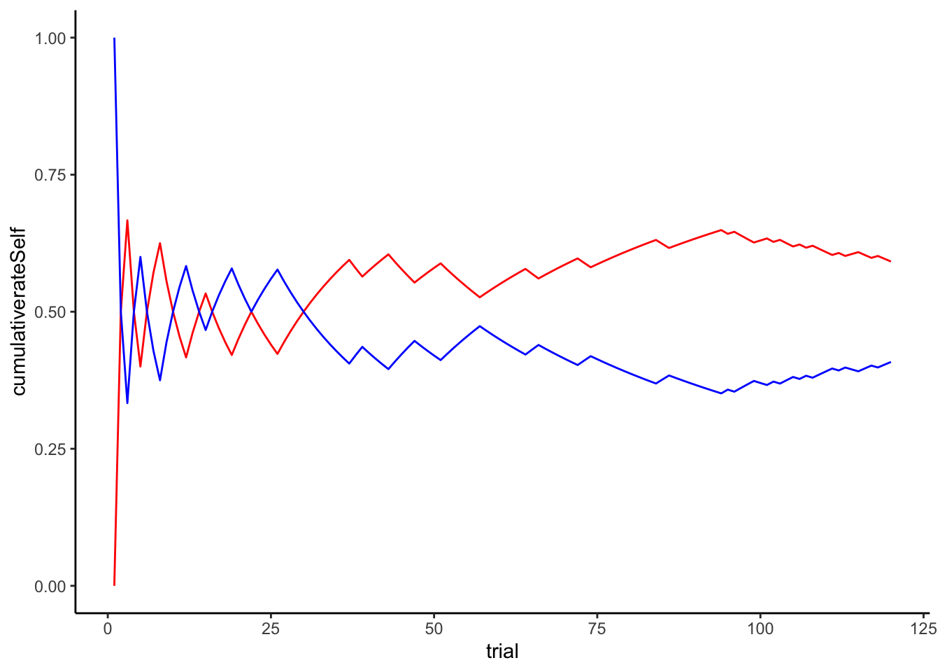
df$cumulativerateSelf <- cumsum(df$Feedback) / seq_along(df$Feedback)
df$cumulativerateOther <- cumsum(1 - df$Feedback) / seq_along(df$Feedback)

ggplot(df) + theme_classic() +
  geom_line(color = "red", aes(trial, cumulativerateSelf)) +
  geom_line(color = "blue", aes(trial, cumulativerateOther))  +
  labs(
    title = "WSLS Agent (red) vs Biased Random Opponent (blue)",
    x = "Trial Number",
    y = "Cumulative probability of choosing 1 (0-1)",
    color = "Agent Type"
  )
# Against a Win-Stay-Lose Shift
Self <- rep(NA, trials)
Other <- rep(NA, trials)

Self[1] <- RandomAgent_f(1, 0.5)
Other[1] <- RandomAgent_f(1, 0.5)

for (i in 2:trials) {
  if (Self[i - 1] == Other[i - 1]) {
    Feedback = 1
  } else {Feedback = 0}
  Self[i] <- WSLSAgent_f(Self[i - 1], Feedback)
  Other[i] <- WSLSAgent_f(Other[i - 1], 1 - Feedback)
}

sum(Self == Other)
## [1] 60df <- tibble(Self, Other, trial = seq(trials), Feedback = as.numeric(Self == Other))
ggplot(df) + theme_classic() +
geom_line(color = "red", aes(trial, Self)) +
geom_line(color = "blue", aes(trial, Other))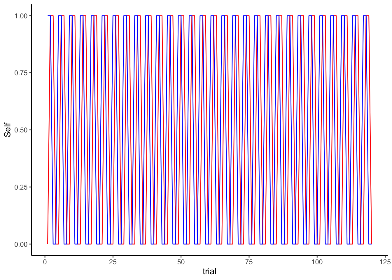
ggplot(df) + theme_classic() +
  geom_line(color = "red", aes(trial, Feedback)) +
  geom_line(color = "blue", aes(trial, 1 - Feedback))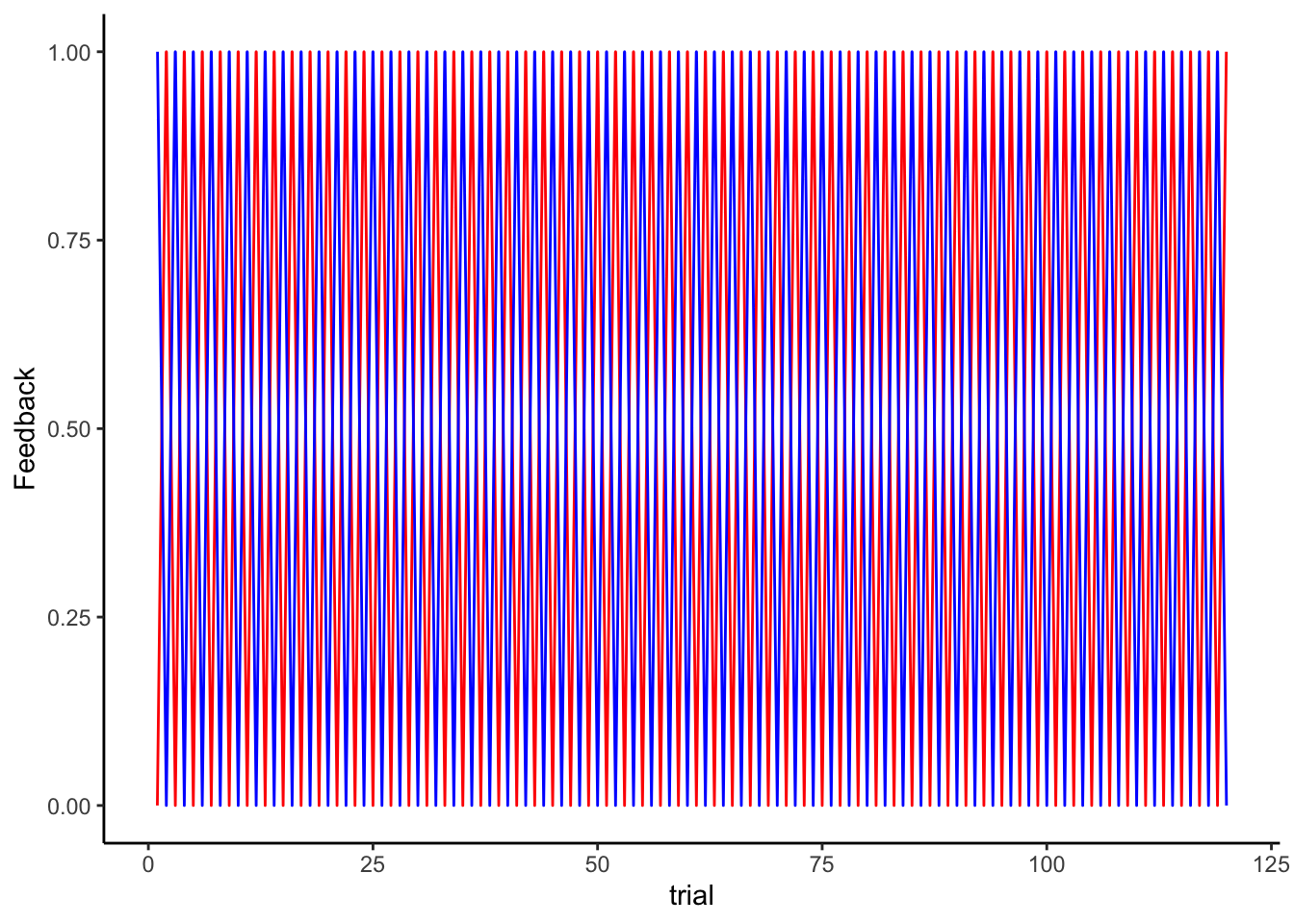
df$cumulativerateSelf <- cumsum(df$Feedback) / seq_along(df$Feedback)
df$cumulativerateOther <- cumsum(1 - df$Feedback) / seq_along(df$Feedback)

ggplot(df) + theme_classic() +
  geom_line(color = "red", aes(trial, cumulativerateSelf)) +
  geom_line(color = "blue", aes(trial, cumulativerateOther))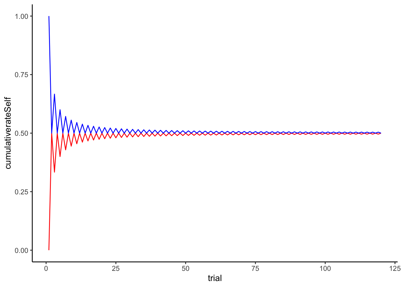
3.5 Now we scale it up
trials = 120
agents = 100

# WSLS vs agents with varying rates

for (rate in seq(from = 0.5, to = 1, by = 0.05)) {

  for (agent in seq(agents)) {
    Self <- rep(NA, trials)
    Other <- rep(NA, trials)

    Self[1] <- RandomAgent_f(1, 0.5)
    Other <- RandomAgent_f(seq(trials), rate)


    for (i in 2:trials) {
      if (Self[i - 1] == Other[i - 1]) {
        Feedback = 1
      } else {Feedback = 0}
      Self[i] <- WSLSAgent_f(Self[i - 1], Feedback)
    }

    temp <- tibble(Self, Other, trial = seq(trials), Feedback = as.numeric(Self == Other), agent, rate)

    if (agent == 1 & rate == 0.5) {df <- temp} else {df <- bind_rows(df, temp)}
  }
}

## WSLS with another WSLS

for (agent in seq(agents)) {
    Self <- rep(NA, trials)
    Other <- rep(NA, trials)

    Self[1] <- RandomAgent_f(1, 0.5)
    Other[1] <- RandomAgent_f(1, 0.5)


    for (i in 2:trials) {
      if (Self[i - 1] == Other[i - 1]) {
        Feedback = 1
      } else {Feedback = 0}
      Self[i] <- WSLSAgent_f(Self[i - 1], Feedback)
      Other[i] <- WSLSAgent_f(Other[i - 1], 1 - Feedback)
    }

    temp <- tibble(Self, Other, trial = seq(trials), Feedback = as.numeric(Self == Other), agent, rate)

    if (agent == 1 ) {df1 <- temp} else {df1 <- bind_rows(df1, temp)}
  }
3.5.1 And we visualize it
ggplot(df, aes(trial, Feedback, group = rate, color = rate)) +
  geom_smooth(se = F) + theme_classic()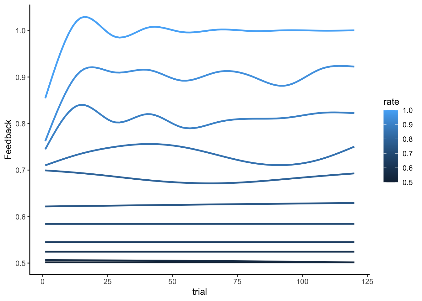
We can see that the bigger the bias in the random agent, the bigger the performance in the WSLS (the higher the chances the random agent picks the same hand more than once in a row).
Now it’s your turn to follow a similar process for your 2 chosen strategies.