Chapter 4 Practical exercise 3 - Getting into Stan
4.1 Overview
The goal of the practical exercise is to build on the simulated data from Practical Exercise 2 to construct our Stan models of the generative processes of the data. Here we know the truth: we simulated the data ourselves, so we can assess how accurate the model is in reconstructing, e.g. the bias of the agents.
4.2 Simulating data
Here we build a new simulation of random agents with bias and noise. The code and visualization is really nothing different from last week’s exercise.
pacman::p_load(tidyverse,
        here,
        posterior,
        cmdstanr,
        brms, tidybayes)

trials <- 120

RandomAgentNoise_f <- function(rate, noise) {

  choice <- rbinom(1, 1, rate) # generating noiseless choices

  if (rbinom(1, 1, noise) == 1) {
    choice = rbinom(1, 1, 0.5) # introducing noise
  }

  return(choice)
}

d <- NULL
for (noise in seq(0, 0.5, 0.1)) { # looping through noise levels

  for (rate in seq(0, 1, 0.1)) { # looping through rate levels
    randomChoice <- rep(NA, trials)

    for (t in seq(trials)) { # looping through trials (to make it homologous to more reactive models)
      randomChoice[t] <- RandomAgentNoise_f(rate, noise)
    }
    temp <- tibble(trial = seq(trials), choice = randomChoice, rate, noise)
    temp$cumulativerate <- cumsum(temp$choice) / seq_along(temp$choice)

    if (exists("d")) {
      d <- rbind(d, temp)
    } else{
      d <- temp
    }
  }
}

write_csv(d, "simdata/W3_randomnoise.csv")

# Now we visualize it
p1 <- ggplot(d, aes(trial, cumulativerate, group = rate, color = rate)) +
  geom_line() +
  geom_hline(yintercept = 0.5, linetype = "dashed") +
  ylim(0,1) +
  facet_wrap(.~noise) +
  theme_classic()
p1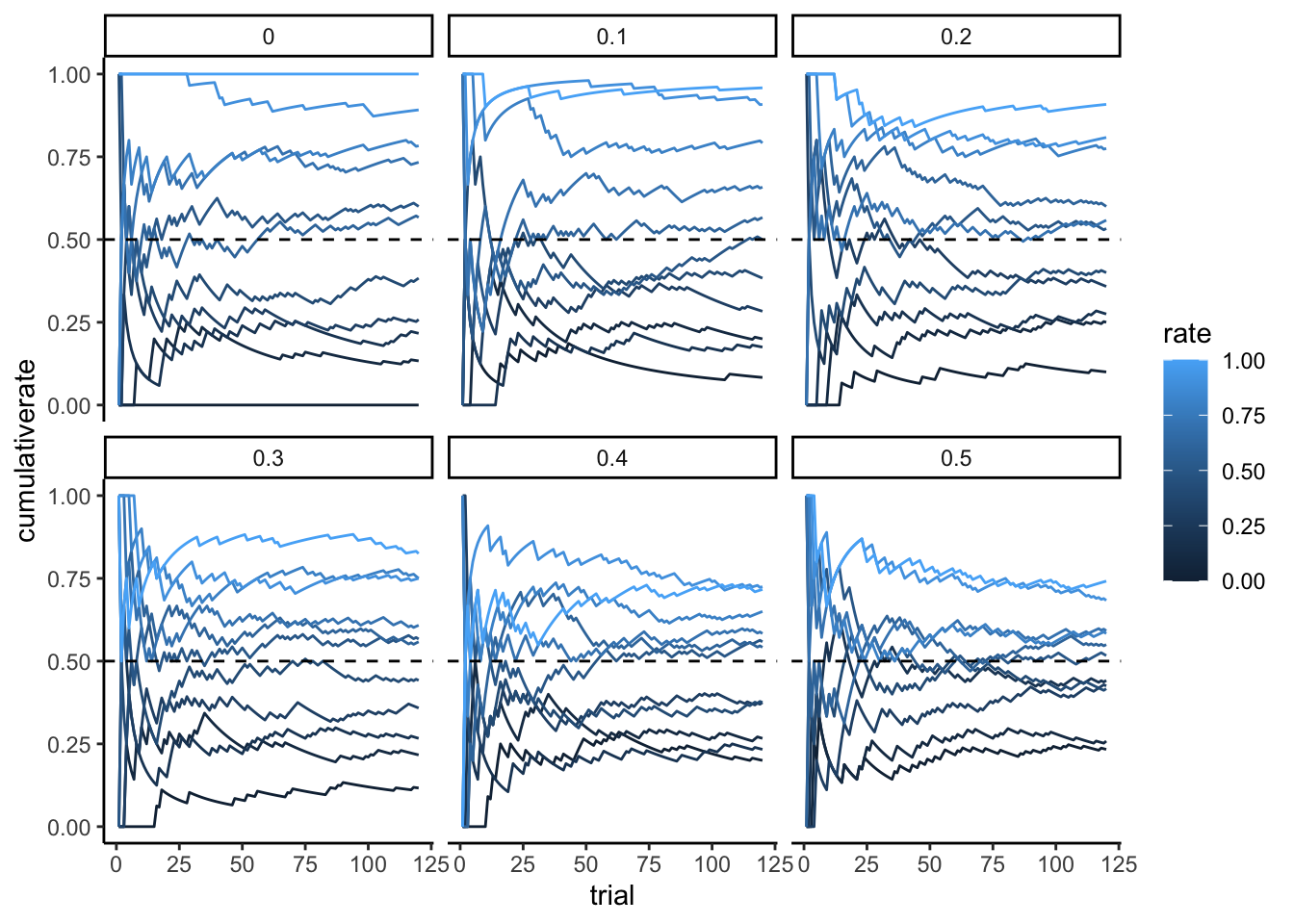
4.3 Building our basic model in Stan
N.B. Refer to the video and slides for the step by step build-up of the Stan code.
Now we subset to a simple case, no noise and rate of 0.8, to focus on the Stan model. We make it into the right format for Stan, build the Stan model, and fit it.
4.3.1 Data
Here we define the data and format it for Stan. Stan likes data as a list. Why a list? Well, dataframes (now tibbles) are amazing. But they have a big drawback: they require each variable to have the same length. Lists do not have that limitation, they are more flexible. So, lists. We’ll have to learn how to live with them.
4.3.2 Model
We write the stan code within the R code (so I can show it to you more easily), then we save it as a stan file, which can be loaded at a later stage in order to compile it. [Missing: more info on compiling etc.]
Remember that the minimal Stan model requires 3 chunks, one specifying the data it will need as input; one specifying the parameters to be estimated; one specifying the model within which the parameters appear, and the priors for those parameters.
stan_model <- "
// This model infers a random bias from a sequences of 1s and 0s (right and left hand choices)

// The input (data) for the model. n of trials and the sequence of choices (right as 1, left as 0)
data {
 int<lower=1> n; // n of trials
 array[n] int h; // sequence of choices (right as 1, left as 0) as long as n
}

// The parameters that the model needs to estimate (theta)
parameters {
  real<lower=0, upper=1> theta; // rate or theta is a probability and therefore bound between 0 and 1
}

// The model to be estimated (a bernoulli, parameter theta, prior on the theta)
model {
  // The prior for theta is a beta distribution alpha of 1, beta of 1, equivalent to a uniform between 0 and 1
  target += beta_lpdf(theta | 1, 1);
  // N.B. you could also define the parameters of the priors as variables to be found in the data
  // target += beta_lpdf(theta | beta_alpha, beta_beta); BUT remember to add beta_alpha and beta_beta to the data list

  // The model consists of a bernoulli distribution (binomial w 1 trial only) with a rate theta
  target += bernoulli_lpmf(h | theta);
}
"
write_stan_file(
  stan_model,
  dir = "stan/",
  basename = "W3_SimpleBernoulli.stan")
4.3.3 Compiling and fitting the model
## Specify where the model is
file <- file.path("stan/W3_SimpleBernoulli.stan")

# Compile the model
mod <- cmdstan_model(file,
                     # this specifies we can parallelize the gradient estimations on multiple cores
                     cpp_options = list(stan_threads = TRUE),
                     # this is a trick to make it faster
                     stanc_options = list("O1"))

# The following command calls Stan with specific options.
samples <- mod$sample(
  data = data, # the data :-)
  seed = 123,  # a seed, so I always get the same results
  chains = 2,  # how many chains should I fit (to check whether they give the same results)
  parallel_chains = 2, # how many of the chains can be run in parallel?
  threads_per_chain = 2, # distribute gradient estimations within chain across multiple cores
  iter_warmup = 1000,  # warmup iterations through which hyperparameters (steps and step length) are adjusted
  iter_sampling = 2000, # total number of iterations
  refresh = 0,  # how often to show that iterations have been run
  output_dir = "simmodels", # saves the samples as csv so it can be later loaded
  max_treedepth = 20, # how many steps in the future to check to avoid u-turns
  adapt_delta = 0.99, # how high a learning rate to adjust hyperparameters during warmup
)

# Same the fitted model
samples$save_object("simmodels/W3_SimpleBernoulli.rds")
4.3.4 Summarizing the model
Now the model is ready to be assessed. First we simply generate a summary of the estimates to have a first idea.
## # A tibble: 2 × 10
##   variable    mean  median     sd    mad      q5     q95  rhat ess_bulk
##   <chr>      <dbl>   <dbl>  <dbl>  <dbl>   <dbl>   <dbl> <dbl>    <dbl>
## 1 lp__     -65.0   -64.7   0.711  0.332  -66.4   -64.5    1.00    1417.
## 2 theta      0.776   0.778 0.0384 0.0388   0.709   0.835  1.00     942.
## # ℹ 1 more variable: ess_tail <dbl>
4.3.5 Assessing model quality
Then we need to look more in the details at the quality of the estimation: * the markov chains * how the prior and the posterior estimates relate to each other (whether the prior is constraining the posterior estimate)
# Extract posterior samples and include sampling of the prior:
draws_df <- as_draws_df(samples$draws())

# Checking the model's chains
ggplot(draws_df, aes(.iteration, theta, group = .chain, color = .chain)) +
  geom_line() +
  theme_classic()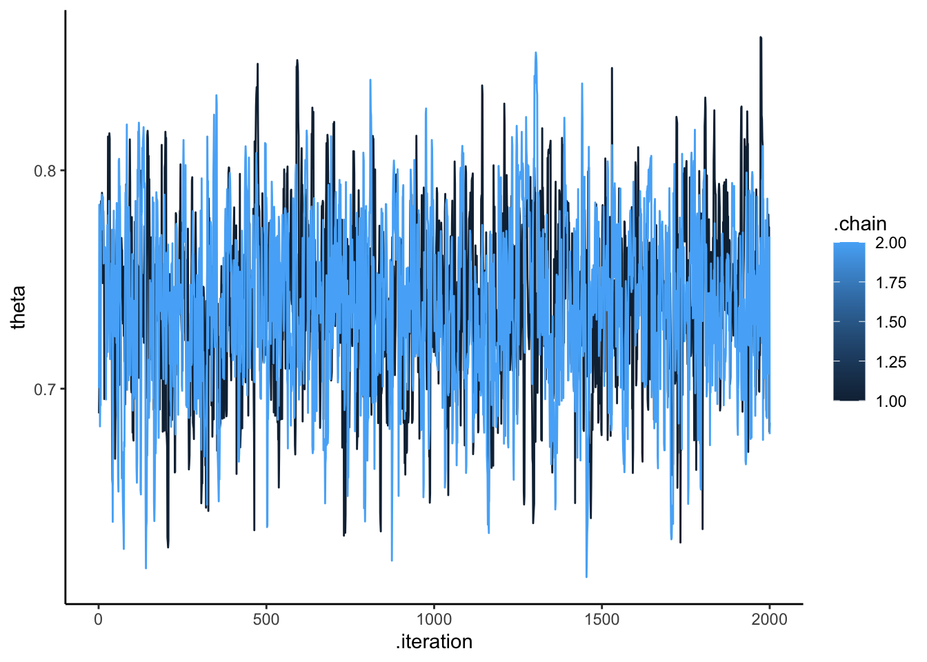
# add a prior for theta (ugly, but we'll do better soon)
draws_df <- draws_df %>% mutate(
  theta_prior = rbeta(nrow(draws_df), 1, 1)
)

# Now let's plot the density for theta (prior and posterior)
ggplot(draws_df) +
  geom_density(aes(theta), fill = "blue", alpha = 0.3) +
  geom_density(aes(theta_prior), fill = "red", alpha = 0.3) +
  geom_vline(xintercept = 0.8, linetype = "dashed", color = "black", linewidth = 1.5) +
  xlab("Rate") +
  ylab("Posterior Density") +
  theme_classic()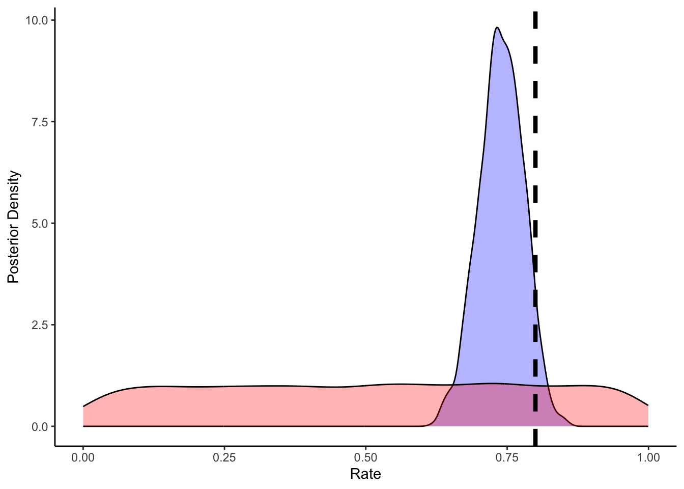
As we can see from the posterior estimates and the prior posterior update check, our model is doing a decent job. It doesn’t exactly reconstruct the rate of 0.8, but 0.755 is pretty close and 0.8 is included within the credible interval.
Now we build the same model, but using the log odds scale for the theta parameter, which will become useful later when we condition theta on variables and build multilevel models (as we can do what we want in a log odds space and it will always be bound between 0 and 1).
stan_model <- "
// This model infers a random bias from a sequences of 1s and 0s (right and left hand choices)

// The input (data) for the model. n of trials and the sequence of choices (right as 1, left as 0)
data {
 int<lower=1> n; // n of trials
 array[n] int h; // sequence of choices (right as 1, left as 0) as long as n
}

// The parameters that the model needs to estimate (theta)
parameters {
    real theta; // note it is unbounded as we now work on log odds
}

// The model to be estimated (a bernoulli, parameter theta, prior on the theta)
model {
  // The prior for theta on a log odds scale is a normal distribution with a mean of 0 and a sd of 1.
  // This covers most of the probability space between 0 and 1, after being converted to probability.
  target += normal_lpdf(theta | 0, 1);
  // as before the parameters of the prior could be fed as variables
  // target += normal_lpdf(theta | normal_mu, normal_sigma);

  // The model consists of a bernoulli distribution (binomial w 1 trial only) with a rate theta,
  // note we specify it uses a logit link (theta is in logodds)
  target += bernoulli_logit_lpmf(h | theta);

}
"
write_stan_file(
  stan_model,
  dir = "stan/",
  basename = "W3_SimpleBernoulli_logodds.stan")
## [1] "/Users/au209589/Dropbox/Teaching/AdvancedCognitiveModeling23_book/stan/W3_SimpleBernoulli_logodds.stan"## With the logit format
## Specify where the model is
file <- file.path("stan/W3_SimpleBernoulli_logodds.stan")
mod <- cmdstan_model(file,
cpp_options = list(stan_threads = TRUE),
stanc_options = list("O1"))
# The following command calls Stan with specific options.
samples <- mod$sample(
data = data,
seed = 123,
chains = 2,
parallel_chains = 2,
threads_per_chain = 2,
iter_warmup = 1000,
iter_sampling = 2000,
refresh = 0,
output_dir = "simmodels",
max_treedepth = 20,
adapt_delta = 0.99,
)## Running MCMC with 2 parallel chains, with 2 thread(s) per chain...
##
## Chain 1 finished in 0.1 seconds.
## Chain 2 finished in 0.0 seconds.
##
## Both chains finished successfully.
## Mean chain execution time: 0.0 seconds.
## Total execution time: 0.2 seconds.4.3.6 Summarizing the results
samples <- readRDS("simmodels/W3_SimpleBernoulli_logodds.rds")
# Diagnostics
samples$cmdstan_diagnose()
## Checking sampler transitions treedepth.
## Treedepth satisfactory for all transitions.
##
## Checking sampler transitions for divergences.
## No divergent transitions found.
##
## Checking E-BFMI - sampler transitions HMC potential energy.
## E-BFMI satisfactory.
##
## Rank-normalized split effective sample size satisfactory for all parameters.
##
## Rank-normalized split R-hat values satisfactory for all parameters.
##
## Processing complete, no problems detected.# Extract posterior samples and include sampling of the prior:
draws_df <- as_draws_df(samples$draws())
ggplot(draws_df, aes(.iteration, theta, group = .chain, color = .chain)) +
geom_line() +
theme_classic()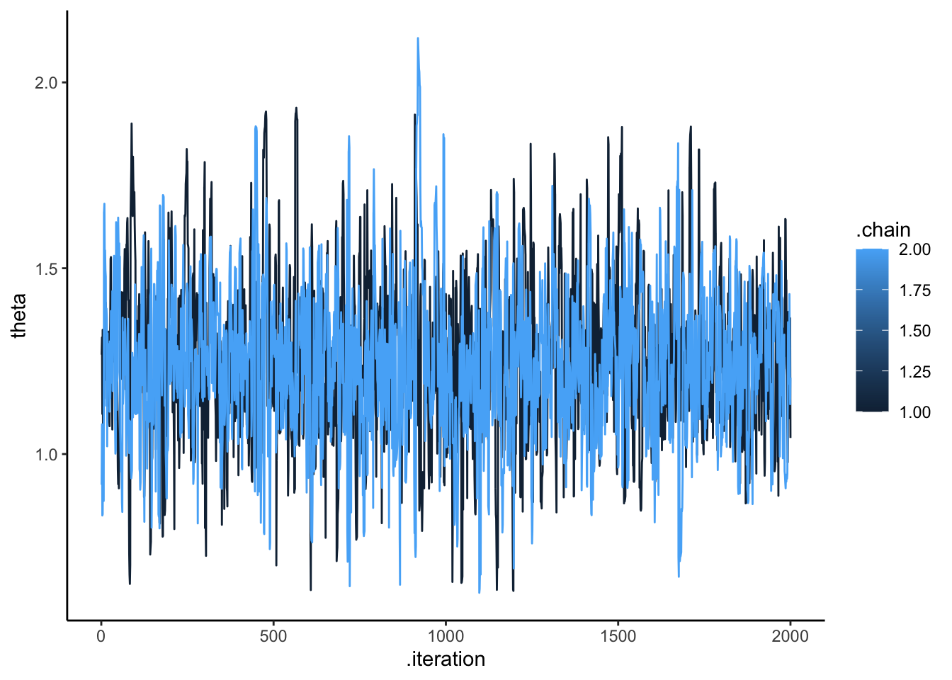
# add a prior for theta (ugly, but we'll do better soon)
draws_df <- draws_df %>% mutate(
theta_prior = rnorm(nrow(draws_df), 0, 1)
)
# Now let's plot the density for theta (prior and posterior)
ggplot(draws_df) +
geom_density(aes(theta), fill = "blue", alpha = 0.3) +
geom_density(aes(theta_prior), fill = "red", alpha = 0.3) +
geom_vline(xintercept = 1.38, linetype = "dashed", color = "black", size = 1.5) +
xlab("Rate") +
ylab("Posterior Density") +
theme_classic()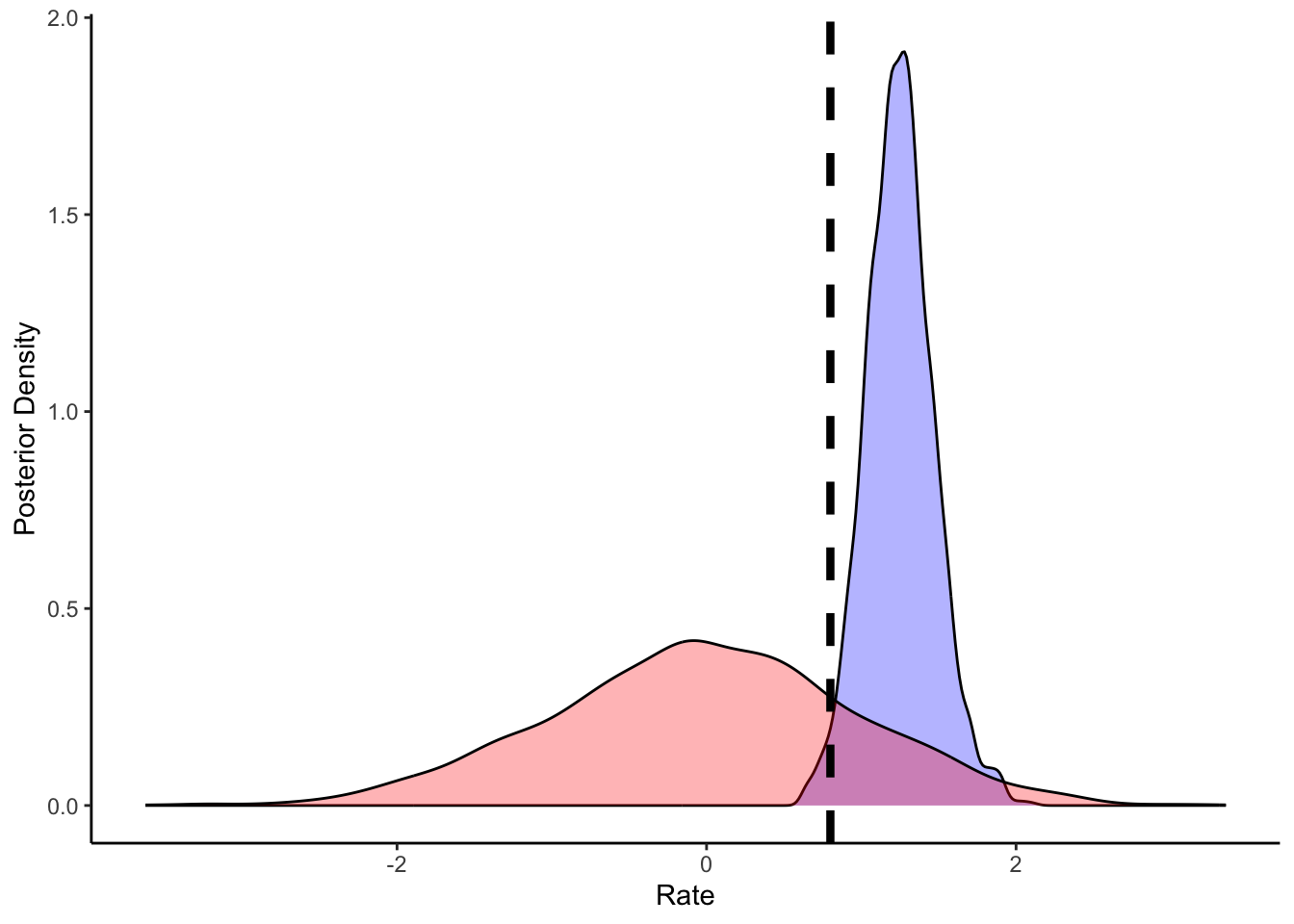
## # A tibble: 2 × 10
## variable mean median sd mad q5 q95 rhat ess_bulk ess_tail
## <chr> <dbl> <dbl> <dbl> <dbl> <dbl> <dbl> <dbl> <dbl> <dbl>
## 1 lp__ -56.7 -56.5 0.710 0.335 -58.2 -56.2 1.00 935. 877.
## 2 theta 1.54 1.53 0.239 0.244 1.16 1.96 1.00 950. 803.We can see that the results are very similar.
4.4 Parameter recovery
Now that we see that the model works in one case, we can run it throughout all possible rate and noise levels in the simulation. N.B. here is using loops, parallelized version in the next code chunk.
# Now we need to scale it up to all possible rates and noises
recovery_df <- NULL
for (noiseLvl in unique(d$noise)) {
for (rateLvl in unique(d$rate)) {
dd <- d %>% subset(
noise == noiseLvl & rate == rateLvl
)
data <- list(
n = 120,
h = dd$choice
)
samples <- mod$sample(
data = data,
seed = 123,
chains = 1,
parallel_chains = 1,
threads_per_chain = 1,
iter_warmup = 1000,
iter_sampling = 2000,
refresh = 0,
max_treedepth = 20,
adapt_delta = 0.99,
)
draws_df <- as_draws_df(samples$draws())
temp <- tibble(biasEst = inv_logit_scaled(draws_df$theta),
biasTrue = rateLvl, noise = noiseLvl)
if (exists("recovery_df")) {recovery_df <- rbind(recovery_df, temp)} else {recovery_df <- temp}
}
}
write_csv(recovery_df, "simdata/W3_recoverydf_simple.csv")Now we can look at the relation between the “true” bias value we inputted in the simulation and the inferred bias value - the posterior estimates of bias.
recovery_df <- read_csv("simdata/W3_recoverydf_simple.csv")
ggplot(recovery_df, aes(biasTrue, biasEst)) +
geom_point(alpha = 0.1) +
geom_smooth() +
facet_wrap(.~noise) +
theme_classic()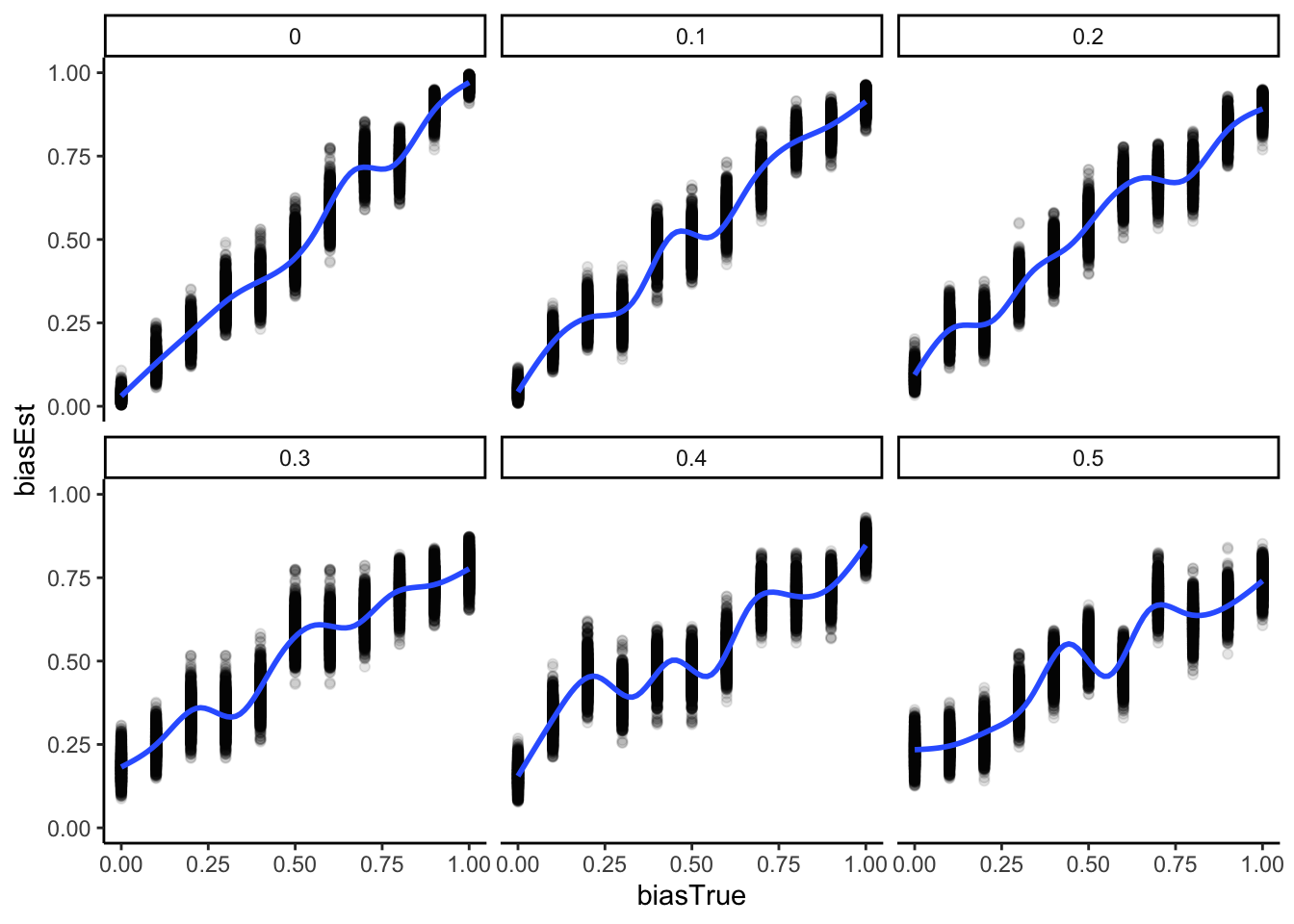
There’s much to be said about the final plot, but for now let’s just say that it looks good. We can reconstruct in a nice ordered way true rate values. However, our ability to do so decreases with the increase in noise. So far no surprises. Wait, you say, shouldn’t we actually model the generative process, that is, include noise in the Stan model? Gold star, there! But let’s wait a bit before we get there, we’ll need mixture models.
One final note before moving to the memory model: what if we parallelized the parameter recovery, so that different models / datasets run on different cores? This was not necessary above (it ran in a few minutes anyway), but will become crucial with more complex models.
To parallelize, we rely on furrr, a neat R package that distributes parallel operations across cores. First we need to define the function that will define the operations to be run on each core separately, here we simulate the data according to a seed, a n of trials, a rate and a noise, and then we fit the model to them. Second, we need to create a tibble of the seeds, n of trials, rate and noise values that should be simulated. Third, we use future_pmap_dfr to run the function on each row of the tibble above separately on a different core. Note that I set the system to split across 4 parallel cores (to work on my computer without clogging it). Do change it according to the system you are using. Note that if you have 40 “jobs” (rows of the tibble, sets of parameter values to run), using e.g. 32 cores will not substantially speed things more than using 20.
pacman::p_load(future, purrr, furrr)
plan(multisession, workers = 4)
sim_d_and_fit <- function(seed, trials, rateLvl, noiseLvl) {
for (t in seq(trials)) { # looping through trials (to make it homologous to more reactive models)
randomChoice[t] <- RandomAgentNoise_f(rateLvl, noiseLvl)
}
temp <- tibble(trial = seq(trials), choice = randomChoice, rate, noise)
data <- list(
n = 120,
h = temp$choice
)
samples <- mod$sample(
data = data,
seed = 1000,
chains = 1,
parallel_chains = 1,
threads_per_chain = 1,
iter_warmup = 1000,
iter_sampling = 2000,
refresh = 0,
max_treedepth = 20,
adapt_delta = 0.99,
)
draws_df <- as_draws_df(samples$draws())
temp <- tibble(biasEst = inv_logit_scaled(draws_df$theta),
biasTrue = rateLvl, noise = noiseLvl)
return(temp)
}
temp <- tibble(unique(d[,c("rate", "noise")])) %>%
mutate(seed = 1000, trials = 120) %>%
rename(rateLvl = rate, noiseLvl = noise)
recovery_df <- future_pmap_dfr(temp, sim_d_and_fit, .options = furrr_options(seed = TRUE))
write_csv(recovery_df, "simdata/W3_recoverydf_parallel.csv")And now we load the data and visualize it as before.
recovery_df <- read_csv("simdata/W3_recoverydf_parallel.csv")
ggplot(recovery_df, aes(biasTrue, biasEst)) +
geom_point(alpha = 0.1) +
geom_smooth() +
facet_wrap(.~noise) +
theme_classic()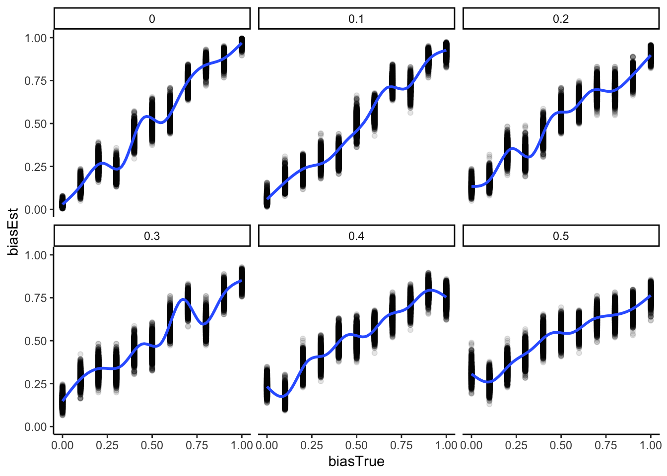
4.5 The memory model: conditioning theta
Now that we fitted the base model, we can move onto more complex models. For instance a memory model (including all previous trials). Here we rely on a generalized linear model kind of thinking: the theta is the expression of a linear model (bias + b1 * PreviousRate). To make the variable more intuitive we code previous rate - which is bound to a probability 0-1 space - into log-odds via a logit link/transformation. In this way a previous rate with more left than right choices will result in a negative value, thereby decreasing our propensity to choose right; and one with more right than left choices will result in a positive value, thereby increasing our propensity to choose right.
# We subset to only include no noise and a specific rate
d1 <- d %>%
subset(noise == 0 & rate == 0.8) %>%
rename(Other = choice) %>%
mutate(cumulativerate = lag(cumulativerate, 1))
d1$cumulativerate[1] <- 0.5 # no prior info at first trial
d1$cumulativerate[d1$cumulativerate == 0] <- 0.01
d1$cumulativerate[d1$cumulativerate == 1] <- 0.99
# Now we create the memory agent with a coefficient of 0.9
MemoryAgent_f <- function(bias, beta, cumulativerate){
choice = rbinom(1, 1, inv_logit_scaled(bias + beta * cumulativerate))
return(choice)
}
d1$Self[1] <- RandomAgentNoise_f(0.5, 0)
for (i in 2:trials) {
d1$Self[i] <- MemoryAgent_f(bias = 0, beta = 0.8, d1$cumulativerate[i])
}
## Create the data
data <- list(
n = 120,
h = d1$Self,
memory = d1$cumulativerate # this creates the new parameter: the rate of right hands so far in log-odds
)stan_model <- "
// The input (data) for the model. n of trials and h for (right and left) hand
data {
int<lower=1> n;
array[n] int h;
vector[n] memory; // here we add the new parameter. N.B. Log odds
}
// The parameters accepted by the model.
parameters {
real bias; // how likely is the agent to pick right when the previous rate has no information (50-50)?
real beta; // how strongly is previous rate impacting the decision?
}
// The model to be estimated.
model {
// priors
target += normal_lpdf(bias | 0, .3);
target += normal_lpdf(beta | 0, .5);
// model
target += bernoulli_logit_lpmf(h | bias + beta * logit(memory));
}
"
write_stan_file(
stan_model,
dir = "stan/",
basename = "W3_MemoryBernoulli.stan")
## Specify where the model is
file <- file.path("stan/W3_MemoryBernoulli.stan")
mod <- cmdstan_model(file, cpp_options = list(stan_threads = TRUE),
stanc_options = list("O1"))
# The following command calls Stan with specific options.
samples <- mod$sample(
data = data,
seed = 123,
chains = 2,
parallel_chains = 2,
threads_per_chain = 2,
iter_warmup = 1000,
iter_sampling = 1000,
refresh = 0,
output_dir = "simmodels",
max_treedepth = 20,
adapt_delta = 0.99,
)
# Same the fitted model
samples$save_object("simmodels/W3_MemoryBernoulli.rds")4.5.1 Summarizing the results
## Checking sampler transitions treedepth.
## Treedepth satisfactory for all transitions.
##
## Checking sampler transitions for divergences.
## No divergent transitions found.
##
## Checking E-BFMI - sampler transitions HMC potential energy.
## E-BFMI satisfactory.
##
## Rank-normalized split effective sample size satisfactory for all parameters.
##
## Rank-normalized split R-hat values satisfactory for all parameters.
##
## Processing complete, no problems detected.
# Extract posterior samples and include sampling of the prior:
draws_df <- as_draws_df(samples$draws())
ggplot(draws_df, aes(.iteration, bias, group = .chain, color = .chain)) +
geom_line() +
theme_classic()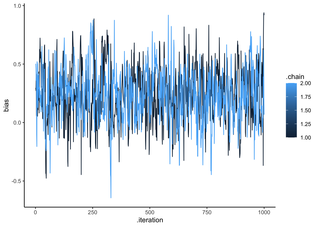
ggplot(draws_df, aes(.iteration, beta, group = .chain, color = .chain)) +
  geom_line() +
  theme_classic()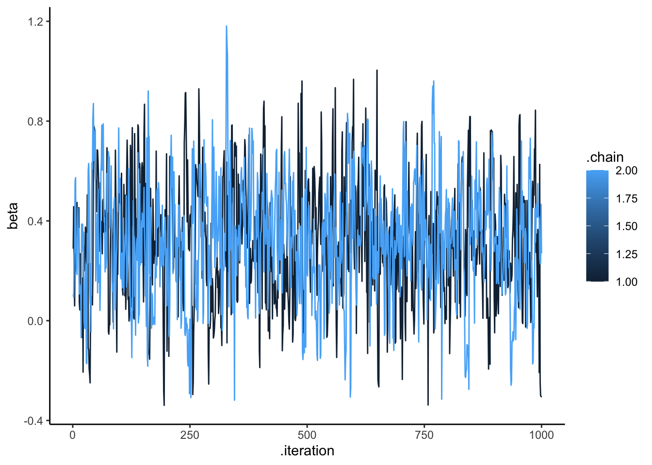
# add a prior for theta (ugly, but we'll do better soon)
draws_df <- draws_df %>% mutate(
  bias_prior = rnorm(nrow(draws_df), 0, .3),
  beta_prior = rnorm(nrow(draws_df), 0, .5),
)

# Now let's plot the density for theta (prior and posterior)
ggplot(draws_df) +
  geom_density(aes(bias), fill = "blue", alpha = 0.3) +
  geom_density(aes(bias_prior), fill = "red", alpha = 0.3) +
  geom_vline(xintercept = 0, linetype = "dashed", color = "black", size = 1.5) +
  xlab("Bias") +
  ylab("Posterior Density") +
  theme_classic()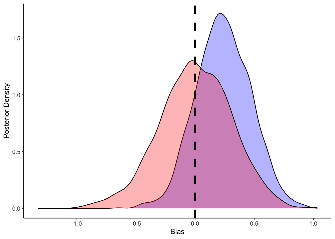
ggplot(draws_df) +
  geom_density(aes(beta), fill = "blue", alpha = 0.3) +
  geom_density(aes(beta_prior), fill = "red", alpha = 0.3) +
  geom_vline(xintercept = 0.8, linetype = "dashed", color = "black", size = 1.5) +
  xlab("Beta") +
  ylab("Posterior Density") +
  theme_classic()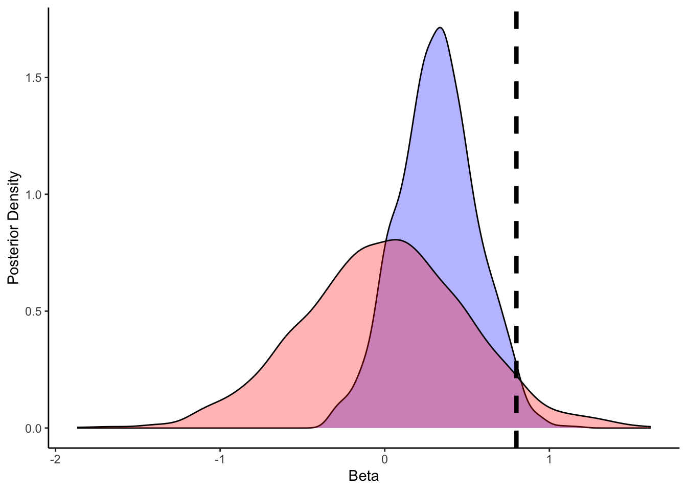
## # A tibble: 3 × 10
##   variable    mean  median    sd   mad       q5     q95  rhat ess_bulk
##   <chr>      <dbl>   <dbl> <dbl> <dbl>    <dbl>   <dbl> <dbl>    <dbl>
## 1 lp__     -78.7   -78.4   1.02  0.734 -80.7    -77.8    1.01     564.
## 2 bias       0.239   0.235 0.230 0.236  -0.130    0.616  1.00     528.
## 3 beta       0.318   0.321 0.239 0.234  -0.0679   0.719  1.00     600.
## # ℹ 1 more variable: ess_tail <dbl>
We can see that the model has now estimated both the bias and the role of previous memory. Bias should reflect the bias in the setup (0.5 which in log odds is 0), and the beta coefficient for memory (roughly 0.8). More on the quality checks of the models in the next chapter.
4.6 Memory agent with internal parameter
So far we behaved like in GLM: we keep feeding to the model an external variable of memory, but what if we coded memory as an internal parameter? This opens up to further possibilities to model how long memory is kept and weighted by distance from the current moment, etc.
[Missing: discussion of the equation of the model, how it relates to Kalman filters, Rescorla-Wagner, and hierarchical gaussian filters]
## Create the data
data <- list(
  n = 120,
  h = d1$Self,
  other = d1$Other
)

stan_model <- "
// The input (data) for the model. n of trials and h for (right and left) hand
data {
 int<lower=1> n;
 array[n] int h;
 array[n] int other;
}

// The parameters accepted by the model.
parameters {
  real bias; // how likely is the agent to pick right when the previous rate has no information (50-50)?
  real beta; // how strongly is previous rate impacting the decision?
}

transformed parameters{
  vector[n] memory;

  for (trial in 1:n){
  if (trial == 1) {
    memory[trial] = 0.5;
  }
  if (trial < n){
      memory[trial + 1] = memory[trial] + ((other[trial] - memory[trial]) / trial);
      if (memory[trial + 1] == 0){memory[trial + 1] = 0.01;}
      if (memory[trial + 1] == 1){memory[trial + 1] = 0.99;}
    }
  }
}

// The model to be estimated.
model {
  // Priors
  target += normal_lpdf(bias | 0, .3);
  target += normal_lpdf(beta | 0, .5);

  // Model, looping to keep track of memory
  for (trial in 1:n) {
    target += bernoulli_logit_lpmf(h[trial] | bias + beta * logit(memory[trial]));
  }
}

"
write_stan_file(
  stan_model,
  dir = "stan/",
  basename = "W3_InternalMemory.stan")
## [1] "/Users/au209589/Dropbox/Teaching/AdvancedCognitiveModeling23_book/stan/W3_InternalMemory.stan"## Specify where the model is
file <- file.path("stan/W3_InternalMemory.stan")
mod <- cmdstan_model(file, cpp_options = list(stan_threads = TRUE),
stanc_options = list("O1"))
# The following command calls Stan with specific options.
samples <- mod$sample(
data = data,
seed = 123,
chains = 1,
parallel_chains = 2,
threads_per_chain = 2,
iter_warmup = 1000,
iter_sampling = 1000,
refresh = 0,
max_treedepth = 20,
adapt_delta = 0.99,
)## Running MCMC with 1 chain, with 2 thread(s) per chain...
##
## Chain 1 finished in 0.5 seconds.## # A tibble: 123 × 10
## variable mean median sd mad q5 q95 rhat ess_bulk
## <chr> <dbl> <dbl> <dbl> <dbl> <dbl> <dbl> <dbl> <dbl>
## 1 lp__ -80.2 -79.9 1.02 0.754 -82.2 -7.92e+1 1.00 373.
## 2 bias 0.433 0.423 0.185 0.174 0.118 7.44e-1 1.00 377.
## 3 beta 0.0167 0.0168 0.135 0.138 -0.211 2.33e-1 1.00 413.
## 4 memory[1] 0.5 0.5 0 0 0.5 5 e-1 NA NA
## 5 memory[2] 0.01 0.01 0 0 0.01 1 e-2 NA NA
## 6 memory[3] 0.005 0.005 0 0 0.005 5 e-3 NA NA
## 7 memory[4] 0.00333 0.00333 0 0 0.00333 3.33e-3 NA NA
## 8 memory[5] 0.0025 0.0025 0 0 0.0025 2.5 e-3 NA NA
## 9 memory[6] 0.202 0.202 0 0 0.202 2.02e-1 NA NA
## 10 memory[7] 0.335 0.335 0 0 0.335 3.35e-1 NA NA
## # ℹ 113 more rows
## # ℹ 1 more variable: ess_tail <dbl>Now that we know how to model memory as an internal state, we can play with making the update discount the past, setting a parameter that indicates after how many trials memory is lost, etc.
4.6.1 Trying out a more complex memory model, with a rate of forgetting that exponentially discounts the past
stan_model <- "
// The input (data) for the model. n of trials and h for (right and left) hand
data {
  int<lower=1> n;
  array[n] int h;
  array[n] int other;
}

// The parameters accepted by the model.
parameters {
  real bias; // how likely is the agent to pick right when the previous rate has no information (50-50)?
  real beta; // how strongly is previous rate impacting the decision?
  real<lower=0, upper=1> forgetting;
}

// The model to be estimated.
model {

  vector[n] memory;
  // Priors
  target += beta_lpdf(forgetting | 1, 1);
  target += normal_lpdf(bias | 0, .3);
  target += normal_lpdf(beta | 0, .5);

  // Model, looping to keep track of memory
  for (trial in 1:n) {
    if (trial == 1) {
      memory[trial] = 0.5;
    }
    target += bernoulli_logit_lpmf(h[trial] | bias + beta * logit(memory[trial]));
    if (trial < n){
      memory[trial + 1] = (1 - forgetting) * memory[trial] + forgetting * other[trial];
      if (memory[trial + 1] == 0){memory[trial + 1] = 0.01;}
      if (memory[trial + 1] == 1){memory[trial + 1] = 0.99;}
    }

  }
}
"
write_stan_file(
  stan_model,
  dir = "stan/",
  basename = "W3_InternalMemory2.stan")
## [1] "/Users/au209589/Dropbox/Teaching/AdvancedCognitiveModeling23_book/stan/W3_InternalMemory2.stan"## Specify where the model is
file <- file.path("stan/W3_InternalMemory2.stan")
mod <- cmdstan_model(file, cpp_options = list(stan_threads = TRUE),
stanc_options = list("O1"))
# The following command calls Stan with specific options.
samples <- mod$sample(
data = data,
seed = 123,
chains = 1,
parallel_chains = 2,
threads_per_chain = 2,
iter_warmup = 1000,
iter_sampling = 1000,
refresh = 0,
max_treedepth = 20,
adapt_delta = 0.99,
)## Running MCMC with 1 chain, with 2 thread(s) per chain...
##
## Chain 1 finished in 1.6 seconds.## # A tibble: 4 × 10
## variable mean median sd mad q5 q95 rhat ess_bulk
## <chr> <dbl> <dbl> <dbl> <dbl> <dbl> <dbl> <dbl> <dbl>
## 1 lp__ -80.0 -79.5 1.57 1.06 -83.2 -78.5 1.02 126.
## 2 bias 0.174 0.168 0.213 0.217 -0.168 0.526 1.02 294.
## 3 beta 0.160 0.152 0.151 0.117 -0.00398 0.403 1.01 286.
## 4 forgetting 0.407 0.382 0.230 0.257 0.0456 0.811 1.00 153.
## # ℹ 1 more variable: ess_tail <dbl>