Chapter 8 The Memory Agent: Two Correlated Individual Differences

8.1 Introduction

The Biased Agent established the full Bayesian workflow for a single individual-level parameter: simulate, fit, diagnose, recover, calibrate. It also taught us, the hard way, that the Centered Parameterization fails when population variance is small, and that the Non-Centered Parameterization resolves this by decoupling individual and population parameters geometrically. We proceed to the Memory Agent with both of those lessons in hand.

The Memory Agent is structurally richer. Recall from Chapter 3 its decision rule. On each trial \(i\), agent \(j\) maintains a running average of the opponent’s past choices \(m_{ij}\) and uses it as a predictive signal:

\[h_{ij} \sim \text{Bernoulli}(\text{logit}^{-1}(\alpha_j + \beta_j \cdot \text{logit}(m_{ij})))\]

\[m_{ij} = \frac{1}{i-1}\sum_{k=1}^{i-1} o_{kj}\]

There are now two individual-level parameters per agent: \(\alpha_j\), the baseline directional bias, and \(\beta_j\), the sensitivity to opponent history. They need not vary independently across the population. An agent who has a strong directional tendency might also track the opponent more aggressively — or might not. Fitting two separate univariate hierarchical models forecloses this question before the data can answer it. We model the parameters jointly.

8.1.1 The Bivariate Population Distribution

\[\begin{pmatrix} \alpha_j \\ \beta_j \end{pmatrix} \sim \mathcal{N}_2\!\left(\boldsymbol{\mu},\, \boldsymbol{\Sigma}\right), \quad \boldsymbol{\Sigma} = \operatorname{diag}(\boldsymbol{\sigma})\, \Omega\, \operatorname{diag}(\boldsymbol{\sigma}), \quad \Omega = \begin{pmatrix} 1 & \rho \\ \rho & 1 \end{pmatrix}\]

This decomposition separates how much individuals differ on each cognitive dimension (\(\sigma_\alpha\), \(\sigma_\beta\)) from how those dimensions covary (\(\rho\)). The scalar \(\rho \in (-1, 1)\) is the key new inferential target.

8.1.2 The LKJ Prior

We need a prior on the correlation matrix \(\Omega\). Stan provides the LKJ distribution (Lewandowski, Kurowicka, and Joe, 2009), with a single shape parameter \(\eta > 0\):

\[\Omega \sim \text{LKJ}(\eta) \quad \propto \quad (\det \Omega)^{\eta - 1}\]

When \(\eta = 1\) the distribution is uniform over valid correlation matrices. When \(\eta > 1\) mass concentrates toward the identity, encoding the prior belief that parameters tend to vary independently unless the data argue otherwise. For a \(2 \times 2\) matrix, the marginal on \(\rho\) reduces to a rescaled Beta: \(\rho \sim 2 \cdot \text{Beta}(\eta, \eta) - 1\). With our default \(\eta = 2\), the prior is unimodal at zero and weakly regularizes against extreme correlations.

Stan samples the lower-triangular Cholesky factor \(\mathbf{L}_\Omega\) (declared as cholesky_factor_corr[2]) under the lkj_corr_cholesky(eta) prior, recovering \(\Omega = \mathbf{L}_\Omega \mathbf{L}_\Omega^\top\) in generated quantities. This parameterization is unconstrained on its natural manifold.

8.1.3 Non-Centered Parameterization

The scalar NCP from the biased agent (\(\theta_j = \mu + z_j \cdot \sigma\)) generalizes directly. We introduce a \(2 \times J\) matrix of independent standard normals:

\[z_{kj} \sim \mathcal{N}(0, 1) \text{ i.i.d.}, \qquad \begin{pmatrix}\alpha_j \\ \beta_j\end{pmatrix} = \begin{pmatrix}\mu_\alpha \\ \mu_\beta\end{pmatrix} + \operatorname{diag}(\boldsymbol{\sigma})\,\mathbf{L}_\Omega\,\mathbf{z}_j\]

The sampler traverses the flat, isotropic space of \(\mathbf{Z}\), whose geometry is entirely independent of \(\boldsymbol{\sigma}\) and \(\Omega\). Neal’s Funnel is structurally impossible.

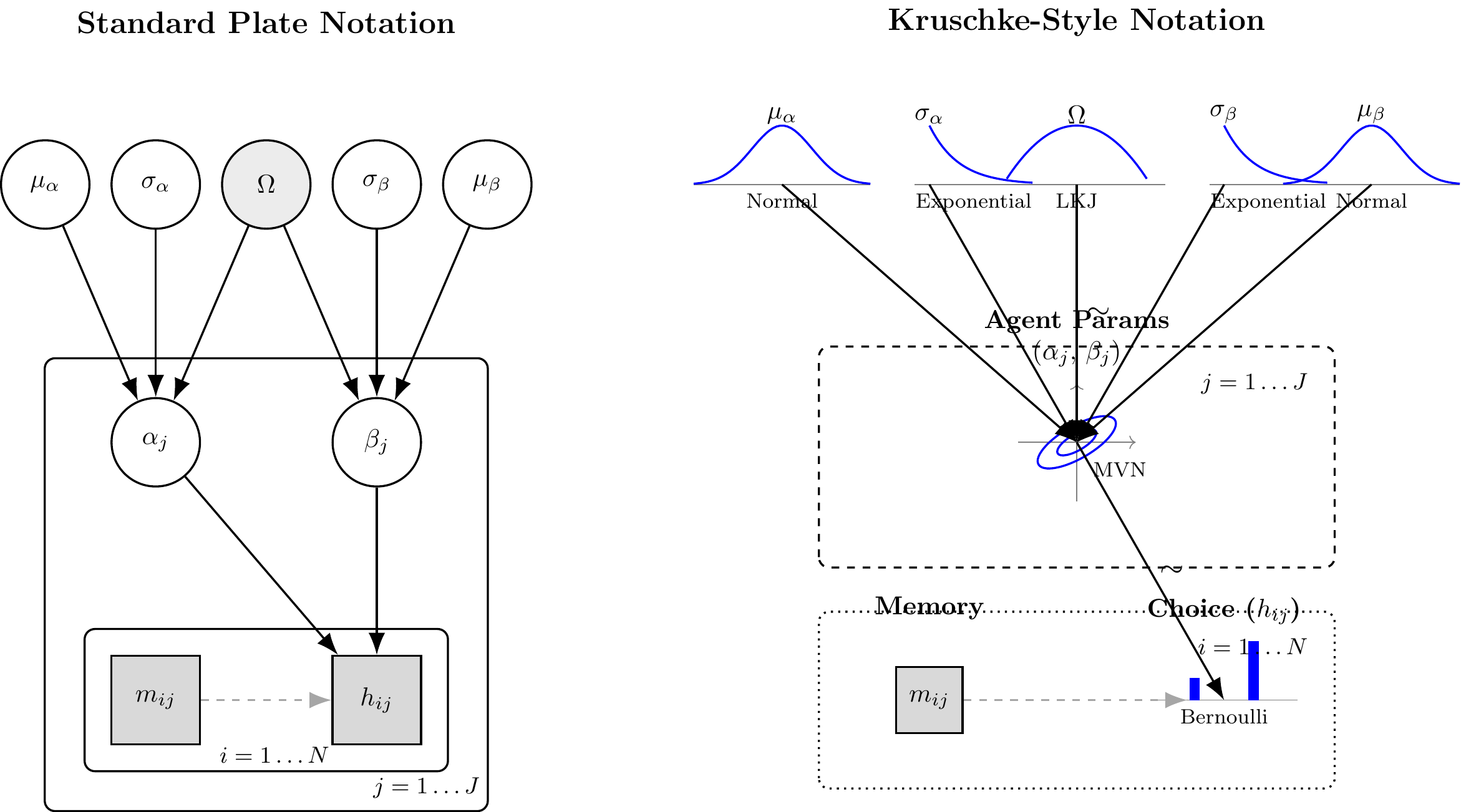
(#fig:hierarchical_memory_dag)Standard Plate Notation (left) and Kruschke-Style Notation (right) for the Hierarchical Memory Agent. The correlation node Omega and the bivariate MVN distinguish this model from the biased agent.

8.2 Phase 1: Generative Plausibility of the Memory Agent

Before writing any Stan code, we construct the forward generative model in R. This code must strictly mirror the mathematical hierarchy above.

One design decision deserves explicit justification. The memory signal \(m_{ij}\) is a deterministic function of the opponent’s past choices. We could compute it inside Stan’s transformed data block, but this executes a nested loop on every leapfrog step of every chain. Instead, we pre-compute the vector opp_rate_prev in R once and pass it as data. This reduces the memory calculation to a single vectorized pass before fitting begins, at zero loss of model fidelity.

The simulation function must also mirror the NCP Stan model exactly. We draw \(\mathbf{z}_j \sim \mathcal{N}(\mathbf{0}, \mathbf{I}_2)\) and apply the Cholesky transform, exactly as the Stan model will. For a \(2 \times 2\) correlation matrix with off-diagonal \(\rho\), the lower Cholesky factor is:

\[\mathbf{L}_\Omega = \begin{pmatrix} 1 & 0 \\ \rho & \sqrt{1-\rho^2} \end{pmatrix}\]

We sample \(\rho\) from the LKJ(2) marginal: \(\rho \sim 2 \cdot \text{Beta}(2, 2) - 1\).

In accordance with the rigorous Bayesian workflow, the simulation function is designed to either:

• Draw all hyperparameters directly from the stated priors (for Prior Predictive Checks).

• Accept fixed ground-truth hyperparameters (for Parameter Recovery).

#' Simulate Hierarchical Memory Agents
#'
#' @param n_agents Integer, number of agents (J).
#' @param n_trials_min Integer, minimum trials per agent.
#' @param n_trials_max Integer, maximum trials per agent.
#' @param mu_alpha Numeric, population mean baseline bias (logit scale). NULL draws from prior.
#' @param mu_beta Numeric, population mean memory sensitivity. NULL draws from prior.
#' @param sigma_alpha Numeric, population SD of alpha. NULL draws from prior.
#' @param sigma_beta Numeric, population SD of beta. NULL draws from prior.
#' @param rho Numeric, population correlation alpha-beta. NULL draws from LKJ(2).
#' @param opponent_rate Numeric, true probability of opponent choosing "right".
#' @param seed Integer, for exact computational reproducibility.
#'
#' @return A tidy tibble containing both latent parameters and observed choices.
simulate_hierarchical_memory <- function(
  n_agents      = 50,
  n_trials_min  = 20,
  n_trials_max  = 120,
  mu_alpha      = NULL,
  mu_beta       = NULL,
  sigma_alpha   = NULL,
  sigma_beta    = NULL,
  rho           = NULL,
  opponent_rate = 0.7,
  seed          = NULL
) {
  if (!is.null(seed)) set.seed(seed)

  # 1. Sample hyperparameters from priors if not provided
  if (is.null(mu_alpha))    mu_alpha    <- rnorm(1, 0, 1)
  if (is.null(mu_beta))     mu_beta     <- rnorm(1, 0, 1)
  if (is.null(sigma_alpha)) sigma_alpha <- rexp(1, 1)
  if (is.null(sigma_beta))  sigma_beta  <- rexp(1, 1)
  # LKJ(2) marginal on rho for 2x2 = 2*Beta(2,2) - 1
  if (is.null(rho))         rho         <- 2 * rbeta(1, 2, 2) - 1

  # 2. Construct the lower-triangular Cholesky factor L_Omega
  L_Omega <- matrix(c(1, rho, 0, sqrt(1 - rho^2)), nrow = 2, ncol = 2)

  # 3. Sample individual parameters via the NCP transform (mirrors Stan exactly)
  # Z is 2 x J; Scale = diag(sigma) %*% L_Omega
  Z            <- matrix(rnorm(2 * n_agents), nrow = 2)
  Scale        <- diag(c(sigma_alpha, sigma_beta)) %*% L_Omega
  # indiv_params is J x 2: column 1 = alpha_j, column 2 = beta_j
  indiv_params <- t(c(mu_alpha, mu_beta) + Scale %*% Z)

  # 4. Simulate trial-level data
  n_trials_vec <- sample(n_trials_min:n_trials_max, n_agents, replace = TRUE)

  sim_data <- map_dfr(seq_len(n_agents), function(j) {
    n_t     <- n_trials_vec[j]
    alpha_j <- indiv_params[j, 1]
    beta_j  <- indiv_params[j, 2]

    opp_choices <- rbinom(n_t, 1, opponent_rate)

    # Pre-compute running opponent rate BEFORE each trial (strict t-1 history).
    # Trial 1 has no history: initialize to 0.5 (uninformative).
    # Clip to [0.01, 0.99] so logit(opp_rate_prev) is always finite.
    opp_rate_prev    <- numeric(n_t)
    opp_rate_prev[1] <- 0.5
    if (n_t > 1) {
      raw_rates         <- cumsum(opp_choices[-n_t]) / seq_len(n_t - 1)
      opp_rate_prev[-1] <- pmax(0.01, pmin(0.99, raw_rates))
    }

    logit_p       <- alpha_j + beta_j * qlogis(opp_rate_prev)
    agent_choices <- rbinom(n_t, 1, plogis(logit_p))

    tibble(
      agent_id      = j,
      trial         = seq_len(n_t),
      n_trials      = n_t,
      choice        = agent_choices,
      opp_rate_prev = opp_rate_prev,
      true_alpha    = alpha_j,
      true_beta     = beta_j
    )
  })

  attr(sim_data, "hyperparameters") <- list(
    mu_alpha    = mu_alpha,    mu_beta     = mu_beta,
    sigma_alpha = sigma_alpha, sigma_beta  = sigma_beta,
    rho         = rho
  )

  sim_data
}

8.2.1 Executing the Prior Predictive Check: The Joint Population Cloud

For a bivariate model, the most revealing prior predictive display is a scatter of individual \((\alpha_j, \beta_j)\) pairs across multiple prior universes. This simultaneously reveals how dispersed individual differences are (\(\sigma_\alpha\), \(\sigma_\beta\)), how correlated the two cognitive dimensions tend to be (\(\rho\)), and whether any prior universe generates implausible populations (e.g., \(|\beta_j| > 8\), meaning the memory signal completely overrides choice).

# Generate 12 prior universes
prior_sims_mem <- map_dfr(1:12, function(sim_id) {
  sim <- simulate_hierarchical_memory(
    n_agents = 80, n_trials_min = 1, n_trials_max = 1,
    seed = sim_id * 13
  )
  hp <- attr(sim, "hyperparameters")
  sim |>
    distinct(agent_id, true_alpha, true_beta) |>
    mutate(simulation_id = paste("Prior Universe", sim_id))
})

ggplot(prior_sims_mem, aes(x = true_alpha, y = true_beta)) +
  geom_point(alpha = 0.4, size = 0.9, color = "steelblue") +
  geom_vline(xintercept = 0, linetype = "dashed", color = "gray60", linewidth = 0.4) +
  geom_hline(yintercept = 0, linetype = "dashed", color = "gray60", linewidth = 0.4) +
  facet_wrap(~simulation_id, ncol = 4) +
  labs(
    title    = "Prior Predictive Checks: Implied Joint Population Distributions",
    subtitle = "Populations generated by mu ~ N(0,1), sigma ~ Exp(1), Omega ~ LKJ(2)",
    x        = expression("Baseline bias  " * alpha[j] * "  (logit scale)"),
    y        = expression("Memory sensitivity  " * beta[j])
  )

A healthy prior generates a range of cloud shapes — some circular (low \(|\rho|\)), some elongated and tilted (high \(|\rho|\)), some compact (low \(\sigma\)), some diffuse (high \(\sigma\)). No prior universe should collapse all agents to a point or place all agents at implausibly extreme values.

8.3 Phase 2: Data Preparation and the NCP Stan Model

Having established from the biased agent workflow that NCP is our default architecture for cognitive tasks with sparse per-agent data, we implement it directly. We skip the Centered Parameterization entirely.

#' Prepare Memory Agent Data for Stan
#'
#' @param sim_data Tibble from simulate_hierarchical_memory().
#' @return A named list formatted for CmdStanR.
prep_stan_data_memory <- function(sim_data) {
  list(
    N             = nrow(sim_data),
    J             = length(unique(sim_data$agent_id)),
    agent         = sim_data$agent_id,
    h             = sim_data$choice,
    opp_rate_prev = sim_data$opp_rate_prev
  )
}

# Execute the preparation on a specifically generated universe for recovery
sim_data_memory <- simulate_hierarchical_memory(
  n_agents      = 50,
  n_trials_min  = 20,
  n_trials_max  = 120,
  mu_alpha      =  0.0,  # No systematic directional baseline
  mu_beta       =  1.5,  # Moderate positive memory tracking
  sigma_alpha   =  0.3,
  sigma_beta    =  0.5,
  rho           =  0.3,  # Mild positive correlation
  opponent_rate =  0.7,
  seed          = 1981
)

stan_data_memory <- prep_stan_data_memory(sim_data_memory)

8.3.1 Stan Model: Hierarchical Memory Agent (NCP)

The only new structural element relative to the biased agent NCP is the bivariate extension. Instead of a scalar \(z_j\), we have a \(2 \times J\) matrix \(\mathbf{Z}\). Instead of scaling by a single \(\sigma\), we apply diag_pre_multiply(sigma, L_Omega) — which computes \(\operatorname{diag}(\boldsymbol{\sigma})\mathbf{L}_\Omega\) and produces the full Cholesky scale matrix encoding both marginal SDs and the correlation structure.

stan_memory_ncp_code <- "
// Hierarchical Memory Agent Model (Non-Centered Parameterization)
// -------------------------------------------------------------------
// alpha_j (baseline bias) and beta_j (memory sensitivity) are jointly
// drawn from a bivariate Normal. NCP decouples sampling geometry from
// the population parameters, preventing Neal's Funnel.

data {
  int<lower=1> N;                          // Total observations across all agents
  int<lower=1> J;                          // Number of agents
  array[N] int<lower=1, upper=J>  agent;   // Agent index per trial
  array[N] int<lower=0, upper=1>  h;       // Observed binary choices
  // Pre-computed running average of opponent choices, clipped to [0.01, 0.99].
  vector<lower=0.01, upper=0.99>[N] opp_rate_prev;
}

parameters {
  // Population-level parameters
  real mu_alpha;              // Population mean baseline bias (logit scale)
  real mu_beta;               // Population mean memory sensitivity
  vector<lower=0>[2] sigma;   // Marginal SDs: sigma[1] = sigma_alpha, sigma[2] = sigma_beta

  // Cholesky factor of the 2x2 correlation matrix. Prior: Omega ~ LKJ(2).
  cholesky_factor_corr[2] L_Omega;

  // Individual-level parameters (NCP): 2 x J matrix of standard normals.
  // Row 1 = alpha offsets, row 2 = beta offsets.
  matrix[2, J] z;
}

transformed parameters {
  // Reconstruct cognitive parameters from z-space via the Cholesky transform.
  // diag_pre_multiply(sigma, L_Omega) = diag(sigma) * L_Omega  (2x2 matrix)
  // Multiplying by z (2xJ) and transposing gives J x 2.
  matrix[J, 2] indiv_params;
  {
    matrix[2, J] deviations = diag_pre_multiply(sigma, L_Omega) * z;
    for (j in 1:J) {
      indiv_params[j, 1] = mu_alpha + deviations[1, j];
      indiv_params[j, 2] = mu_beta  + deviations[2, j];
    }
  }
}

model {
  // Hyperpriors
  target += normal_lpdf(mu_alpha | 0, 1);
  target += normal_lpdf(mu_beta  | 0, 1);
  target += exponential_lpdf(sigma | 1);
  target += lkj_corr_cholesky_lpdf(L_Omega | 2);

  // Individual-level prior (NCP): geometry fully decoupled from population params
  target += std_normal_lpdf(to_vector(z));

  // Likelihood
  vector[N] logit_p;
  for (i in 1:N) {
    logit_p[i] = indiv_params[agent[i], 1]
               + indiv_params[agent[i], 2] * logit(opp_rate_prev[i]);
  }
  target += bernoulli_logit_lpmf(h | logit_p);
}

generated quantities {
  // Recover the full correlation matrix and the scalar rho
  matrix[2, 2] Omega = multiply_lower_tri_self_transpose(L_Omega);
  real rho = Omega[1, 2];

  // Individual parameters on natural scales
  vector[J] alpha    = indiv_params[, 1];
  vector[J] beta_mem = indiv_params[, 2];

  // Prior log-density (required by priorsense)
  real lprior = normal_lpdf(mu_alpha | 0, 1)
              + normal_lpdf(mu_beta  | 0, 1)
              + exponential_lpdf(sigma | 1)
              + lkj_corr_cholesky_lpdf(L_Omega | 2)
              + std_normal_lpdf(to_vector(z));

  // Prior draws for prior-posterior update plots
  real mu_alpha_prior    = normal_rng(0, 1);
  real mu_beta_prior     = normal_rng(0, 1);
  real sigma_alpha_prior = exponential_rng(1);
  real sigma_beta_prior  = exponential_rng(1);
  // LKJ(2) marginal on rho: 2*Beta(2,2) - 1
  real rho_prior         = 2.0 * beta_rng(2.0, 2.0) - 1.0;

  // Predictive checks and pointwise log-likelihood
  vector[N] log_lik;
  array[N] int h_post_rep;
  array[N] int h_prior_rep;

  // Build a prior-drawn population for h_prior_rep
  cholesky_factor_corr[2] L_Omega_prior = lkj_corr_cholesky_rng(2, 2.0);
  vector[2] sigma_prior = [sigma_alpha_prior, sigma_beta_prior]';
  matrix[2, J] z_prior;
  for (j in 1:J) { z_prior[1,j] = normal_rng(0,1); z_prior[2,j] = normal_rng(0,1); }
  matrix[J, 2] indiv_prior;
  {
    matrix[2, J] dev_prior = diag_pre_multiply(sigma_prior, L_Omega_prior) * z_prior;
    for (j in 1:J) {
      indiv_prior[j, 1] = mu_alpha_prior + dev_prior[1, j];
      indiv_prior[j, 2] = mu_beta_prior  + dev_prior[2, j];
    }
  }

  for (i in 1:N) {
    int j = agent[i];
    real lp_post  = indiv_params[j,1] + indiv_params[j,2] * logit(opp_rate_prev[i]);
    real lp_prior = indiv_prior[j,1]  + indiv_prior[j,2]  * logit(opp_rate_prev[i]);

    log_lik[i]     = bernoulli_logit_lpmf(h[i] | lp_post);
    h_post_rep[i]  = bernoulli_logit_rng(lp_post);
    h_prior_rep[i] = bernoulli_logit_rng(lp_prior);
  }
}
"

stan_file_memory_ncp <- here::here("stan", "ch6_multilevel_memory_ncp.stan")
writeLines(stan_memory_ncp_code, stan_file_memory_ncp)
mod_memory_ncp <- cmdstan_model(stan_file_memory_ncp)

Two Stan details are worth noting. First, the local block { matrix[2,J] deviations = ...; } in transformed parameters confines the intermediate matrix to local scope, preventing it from appearing in the parameter output. Second, lkj_corr_cholesky_rng(2, 2.0) in generated quantities draws a full Cholesky factor from the LKJ(2) prior. This is the correct way to generate prior predictive data — unlike the Beta marginal trick, it generalizes to the \(3 \times 3\) case we will need for the WSLS agent.

8.3.2 Fitting the model

fit_memory_path <- here::here("simmodels", "ch6_fit_memory_ncp.rds")

# Initialize at prior means. L_Omega starts at the identity Cholesky (rho = 0).
# This is a neutral, numerically stable starting point for the correlation geometry.
J_val_mem <- stan_data_memory$J
  
  # A 4-chain dumb list for the Memory Model
  init_memory_list <- list(
    list(mu_alpha = rnorm(1, 0, 0.3), mu_beta = rnorm(1, 0, 0.3), sigma = abs(rnorm(2, 0, 0.3)) + 0.1, L_Omega = matrix(c(1, 0, 0, 1), nrow=2), z = matrix(0, nrow=2, ncol=J_val_mem)),
    list(mu_alpha = rnorm(1, 0, 0.3), mu_beta = rnorm(1, 0, 0.3), sigma = abs(rnorm(2, 0, 0.3)) + 0.1, L_Omega = matrix(c(1, 0, 0, 1), nrow=2), z = matrix(0, nrow=2, ncol=J_val_mem)),
    list(mu_alpha = rnorm(1, 0, 0.3), mu_beta = rnorm(1, 0, 0.3), sigma = abs(rnorm(2, 0, 0.3)) + 0.1, L_Omega = matrix(c(1, 0, 0, 1), nrow=2), z = matrix(0, nrow=2, ncol=J_val_mem)),
    list(mu_alpha = rnorm(1, 0, 0.3), mu_beta = rnorm(1, 0, 0.3), sigma = abs(rnorm(2, 0, 0.3)) + 0.1, L_Omega = matrix(c(1, 0, 0, 1), nrow=2), z = matrix(0, nrow=2, ncol=J_val_mem))
  )

if (regenerate_simulations || !file.exists(fit_memory_path)) {
  fit_memory <- mod_memory_ncp$sample(
    data            = stan_data_memory,
    seed            = 123,
    chains          = 4,
    parallel_chains = 4,
    iter_warmup     = 1000,
    iter_sampling   = 1000,
    init            = init_memory_list, 
    adapt_delta     = 0.90,   
    max_treedepth   = 12,
    refresh         = 0
  )
  fit_memory$save_object(fit_memory_path)
} else {
  fit_memory <- readRDS(fit_memory_path)
}

We raise adapt_delta to 0.90. The bivariate NCP is well-behaved globally, but the correlation parameter \(\rho\) introduces a curved direction that can require longer leapfrog trajectories. The higher target acceptance rate forces the dual-averaging algorithm to find a smaller step size, reducing integration error along this direction. If max_treedepth warnings appear (distinct from divergences), raise max_treedepth further — do not raise adapt_delta in response to those.

8.3.3 Assessing the fitting process

Even if the Stan compiler finishes without explicit warnings, our workflow demands that we systematically verify the geometry of the posterior and the efficiency of the sampler.

#fit_memory$cmdstan_diagnose()
fit_memory$diagnostic_summary()

## $num_divergent
## [1] 0 0 0 0
## 
## $num_max_treedepth
## [1] 0 0 0 0
## 
## $ebfmi
## [1] 0.7683105 0.6756634 0.7775092 0.7508324

We are looking for strict zeros in num_divergent. With the NCP, this should hold. Any divergences here are a signal that adapt_delta needs further adjustment, the priors are misspecified, or there is a structural model issue.

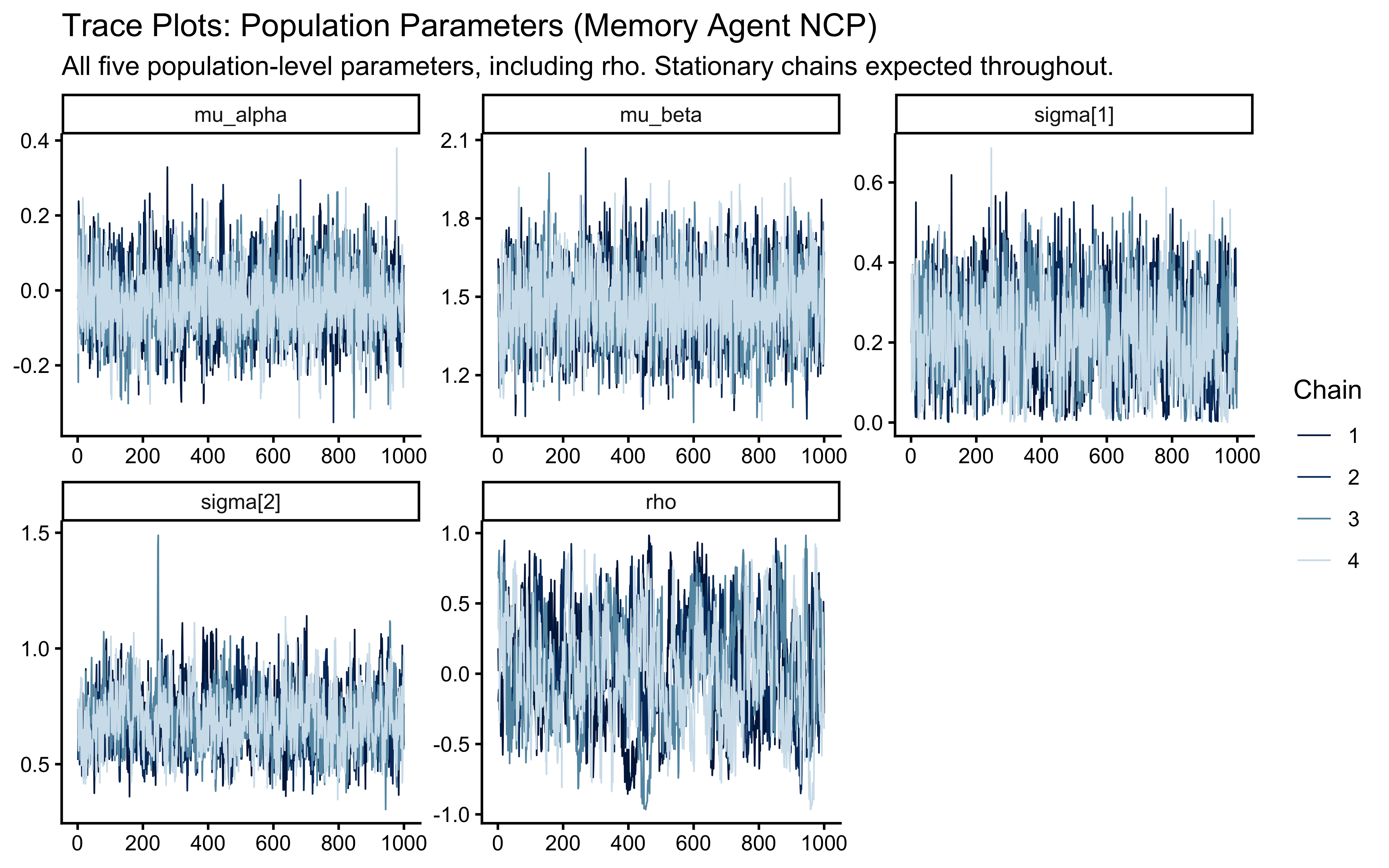
8.3.3.1 Chain Mixing and Stationarity (\(\hat{R}\))

draws_memory <- fit_memory$draws()

mcmc_trace(
  draws_memory,
  pars = c("mu_alpha", "mu_beta", "sigma[1]", "sigma[2]", "rho"),
  np   = nuts_params(fit_memory)
) +
  labs(
    title    = "Trace Plots: Population Parameters (Memory Agent NCP)",
    subtitle = "All five population-level parameters, including rho. Stationary chains expected throughout."
  )

draws_memory |>
  subset_draws(variable = c("mu_alpha", "mu_beta", "sigma[1]", "sigma[2]", "rho",
                            "alpha[1]", "alpha[2]", "beta_mem[1]", "beta_mem[2]")) |>
  summarise_draws(default_convergence_measures()) |>
  knitr::kable(digits = 3)

variable	rhat	ess_bulk	ess_tail
mu_alpha	1.001	1552.332	2308.653
mu_beta	1.002	1738.540	2304.439
sigma[1]	1.006	713.628	940.290
sigma[2]	1.005	600.104	1600.232
rho	1.016	234.634	310.492
alpha[1]	1.000	2054.958	2912.223
alpha[2]	1.004	5550.542	2740.470
beta_mem[1]	1.001	2311.516	3031.242
beta_mem[2]	1.001	5666.282	3009.344

The potential scale reduction factor (\(\hat{R}\)) must be below 1.01 for all parameters. The correlation parameter rho is informed only by covariation across agents, not within any individual agent’s trial sequence, so its ESS will be lower than the marginal parameters. ESS > 400 remains our threshold. An ESS below 200 for rho warrants investigation of the correlation manifold geometry.

8.3.3.2 Effective Sample Size (ESS)

Monitor ess_tail for sigma[1] and sigma[2]. Population SDs can develop mild funnel-like behavior even under NCP when the likelihood is highly informative about individual parameters, because the \(z_j\) draws must simultaneously explain many agents. If ess_tail is low for the sigmas but ess_bulk is acceptable, raising adapt_delta further or running more warmup iterations is the correct response.

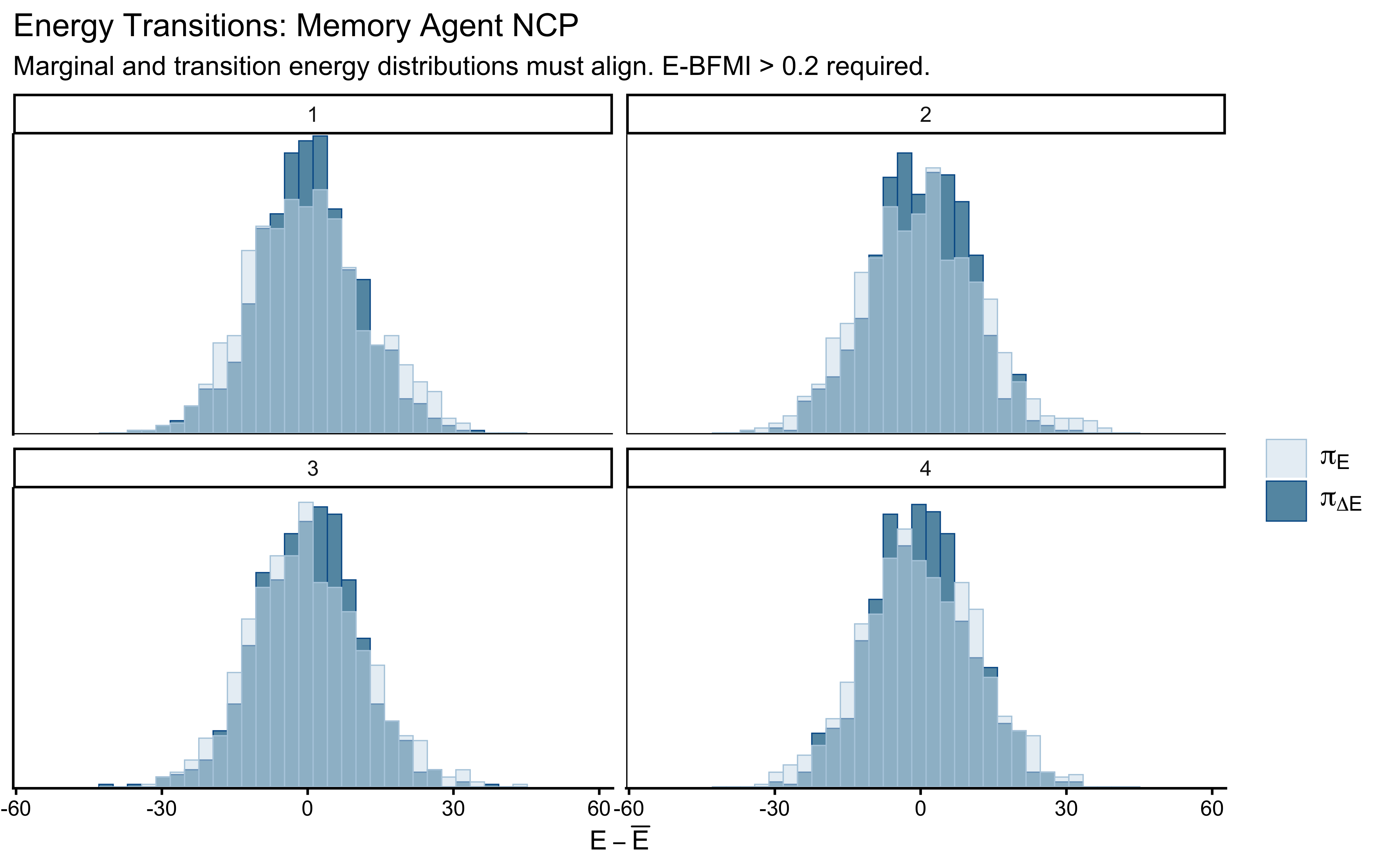
8.3.3.3 Energy (E-BFMI)

mcmc_nuts_energy(nuts_params(fit_memory)) +
  labs(
    title    = "Energy Transitions: Memory Agent NCP",
    subtitle = "Marginal and transition energy distributions must align. E-BFMI > 0.2 required."
  )

8.3.3.4 Posterior Parameter Correlations

mcmc_pairs(
  draws_memory,
  pars         = c("mu_alpha", "mu_beta", "sigma[1]", "sigma[2]", "rho"),
  np           = nuts_params(fit_memory),
  diag_fun     = "dens",
  off_diag_fun = "hex"
)

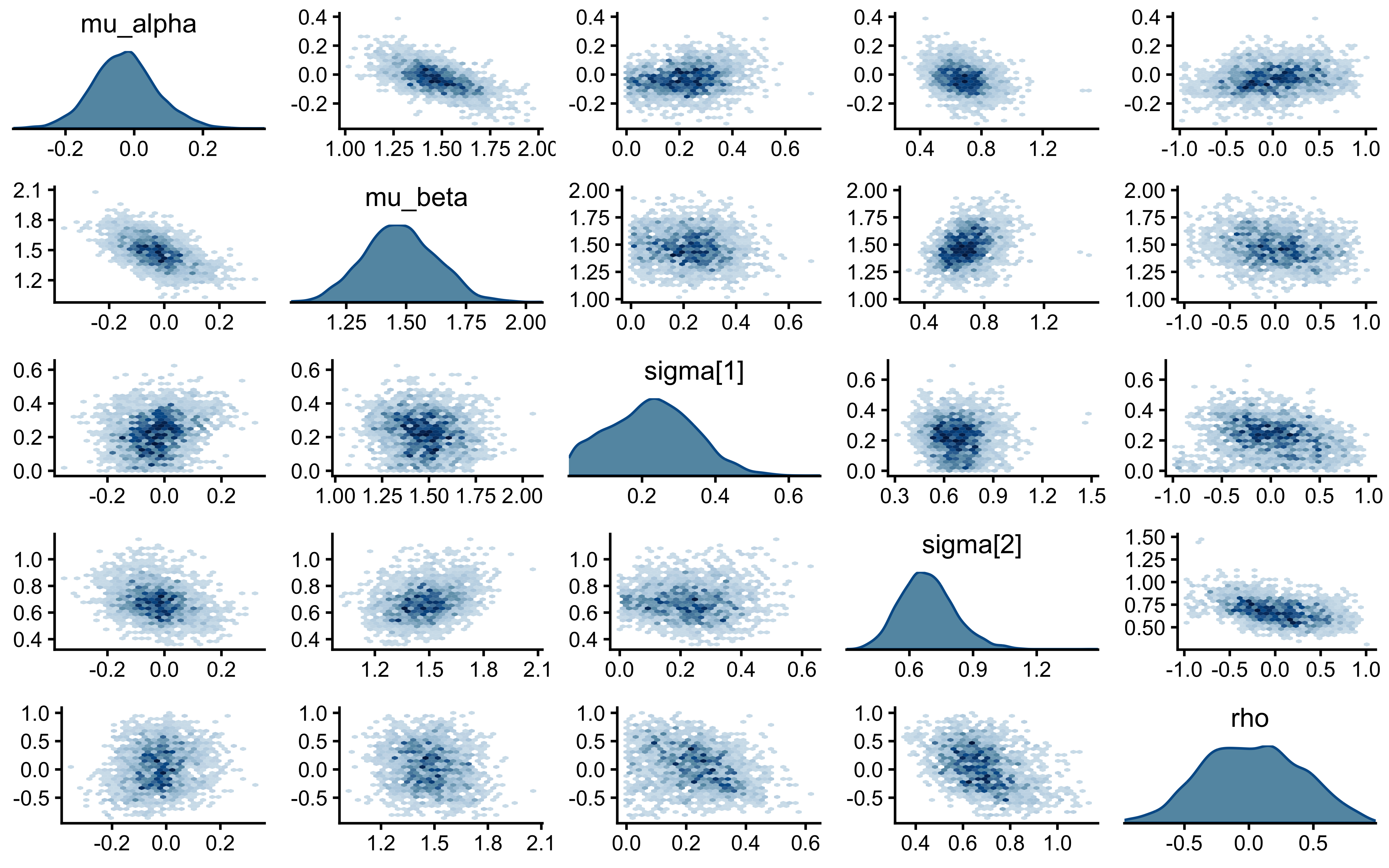
The critical panels are \((\sigma_\alpha, \mu_\alpha)\) and \((\sigma_\beta, \mu_\beta)\). Under the CP biased agent, these showed triangular wedges — the Neal’s Funnel signature. Under NCP, they should be roughly elliptical. Any triangular shape here would be unexpected and would require investigation.

8.3.4 Prior-Posterior Update Checks: Quantifying Learning

draws_df_memory <- as_draws_df(draws_memory)

# Extract true generative hyperparameters saved as attributes
true_hp <- attr(sim_data_memory, "hyperparameters")

true_pop_mem <- tibble(
  parameter  = c("mu_alpha", "mu_beta", "sigma_alpha", "sigma_beta", "rho"),
  true_value = c(true_hp$mu_alpha, true_hp$mu_beta,
                 true_hp$sigma_alpha, true_hp$sigma_beta, true_hp$rho)
)

# Reshape: split on the underscore immediately before "posterior" or "prior"
pp_update_mem <- draws_df_memory |>
  select(
    mu_alpha_posterior  = mu_alpha,        mu_alpha_prior,
    mu_beta_posterior   = mu_beta,         mu_beta_prior,
    sigma_alpha_posterior = `sigma[1]`,    sigma_alpha_prior,
    sigma_beta_posterior  = `sigma[2]`,    sigma_beta_prior,
    rho_posterior       = rho,             rho_prior
  ) |>
  pivot_longer(
    everything(),
    names_to  = c("parameter", "distribution"),
    names_sep = "_(?=posterior|prior)"
  )

ggplot(pp_update_mem, aes(x = value)) +
  geom_histogram(aes(fill = distribution), alpha = 0.6, color = NA, bins = 60) +
  geom_vline(
    data = true_pop_mem,
    aes(xintercept = true_value, linetype = "True Value"),
    color = "darkred", linewidth = 1
  ) +
  facet_wrap(~parameter, scales = "free") +
  scale_fill_manual(
    name   = "Distribution",
    values = c("prior" = "gray70", "posterior" = "steelblue")
  ) +
  scale_linetype_manual(
    name   = "Ground Truth",
    values = c("True Value" = "dashed")
  ) +
  labs(
    title = "Prior-Posterior Update Checks: Memory Agent",
    x     = "Parameter Value",
    y     = "Count"
  )

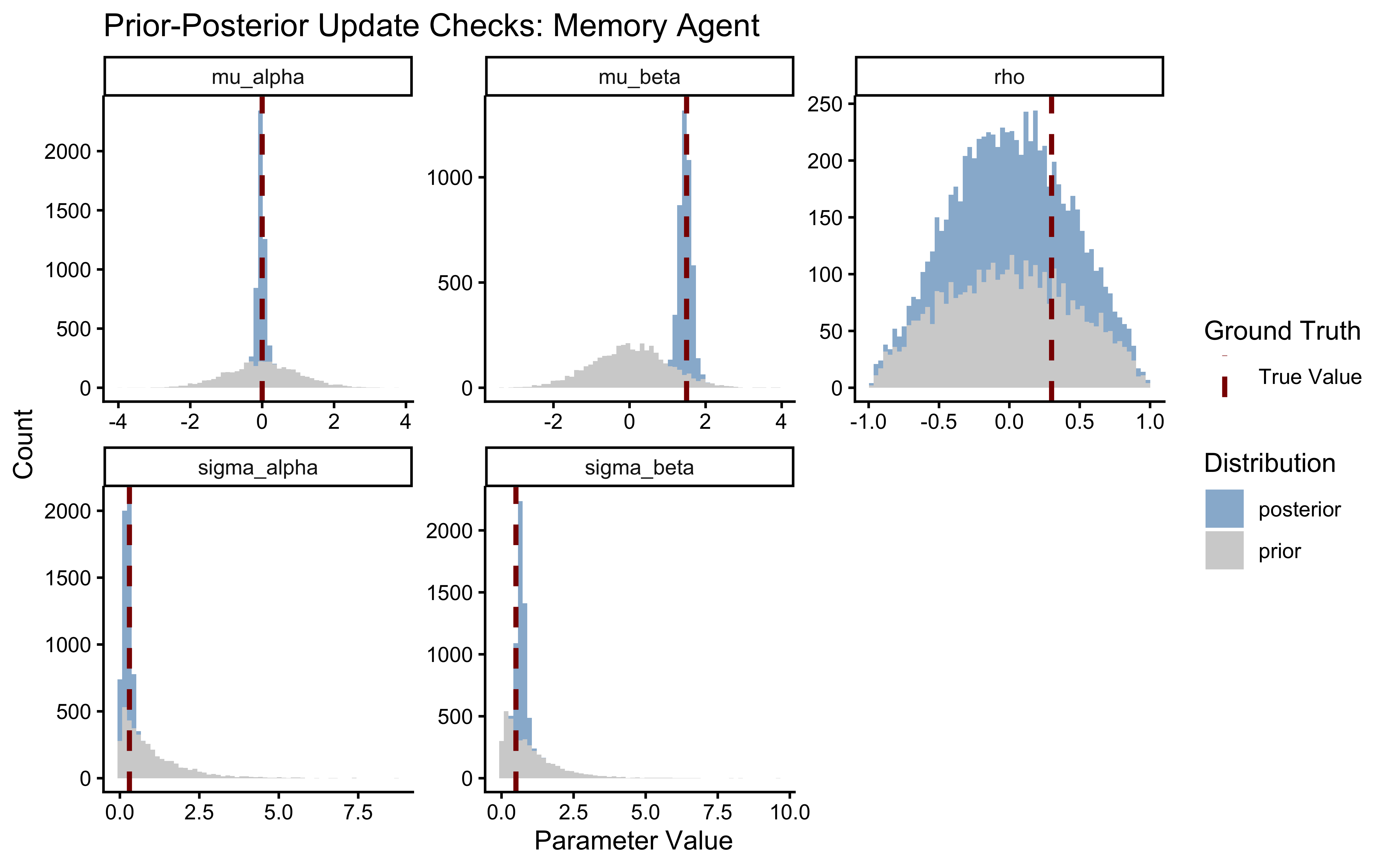
A healthy update shows a posterior significantly narrower than the prior and comfortably contained within the prior’s mass. The rho panel carries the central new scientific information. If the posterior on \(\rho\) is essentially indistinguishable from the LKJ(2) prior, the data do not contain sufficient information to identify the population-level correlation — this can happen with small \(J\) or short trial sequences. In that case, report the parameter as unidentified, not the prior as the conclusion. A clearly narrowed posterior constitutes genuine evidence about the cognitive architecture of the population.

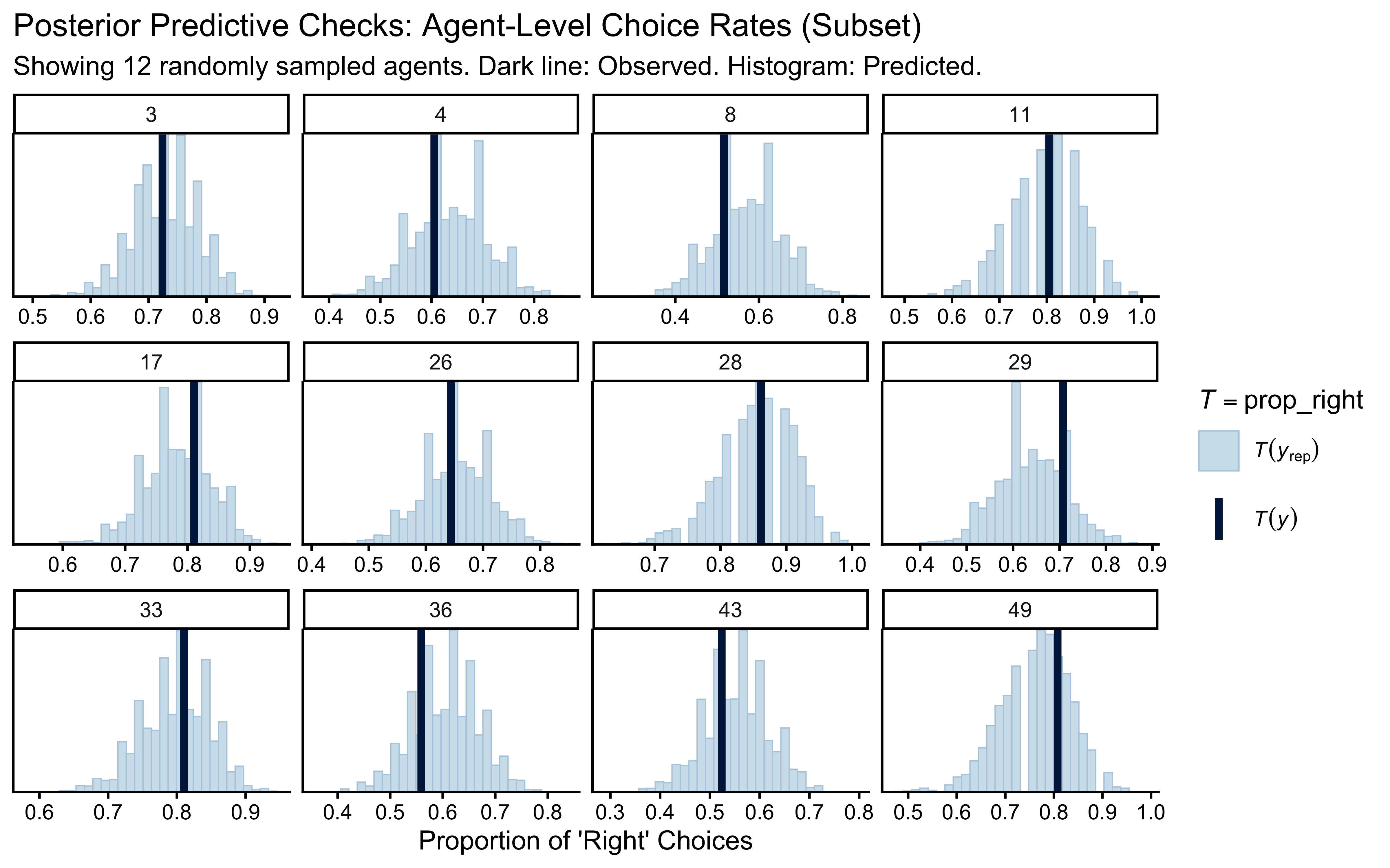
8.3.5 Posterior Predictive Checks (PPC): Generative Adequacy

y_obs_mem     <- as.numeric(stan_data_memory$h)
agent_idx_mem <- as.numeric(stan_data_memory$agent)
y_rep_mem     <- fit_memory$draws("h_post_rep", format = "matrix")

n_sample_mem       <- 12
sampled_agents_mem <- sample(unique(agent_idx_mem), n_sample_mem)
keep_mask_mem      <- agent_idx_mem %in% sampled_agents_mem

prop_right <- function(x) mean(x)

ppc_stat_grouped(
  y     = y_obs_mem[keep_mask_mem],
  yrep  = y_rep_mem[, keep_mask_mem],
  group = agent_idx_mem[keep_mask_mem],
  stat  = "prop_right"
) +
  labs(
    title    = "Posterior Predictive Checks: Agent-Level Choice Rates (Subset)",
    subtitle = paste("Showing", n_sample_mem, "randomly sampled agents. Dark line: Observed. Histogram: Predicted."),
    x        = "Proportion of 'Right' Choices"
  )

8.3.6 Calibration and Recovery

We have proven the model fits the data and generates plausible predictions. Now we must prove the parameters we extract are actually the true parameters that generated the data. For a bivariate model, recovery must be assessed at both levels: all five population parameters, and the individual \((\alpha_j, \beta_j)\) pairs jointly.

8.3.6.1 Individual-Level Recovery

recovery_alpha <- draws_memory |>
  subset_draws(variable = "alpha") |>
  summarise_draws() |>
  mutate(agent_id = as.integer(str_extract(variable, "(?<=\\[)\\d+(?=\\])")))

recovery_beta <- draws_memory |>
  subset_draws(variable = "beta_mem") |>
  summarise_draws() |>
  mutate(agent_id = as.integer(str_extract(variable, "(?<=\\[)\\d+(?=\\])")))

true_agent_params_mem <- sim_data_memory |>
  distinct(agent_id, n_trials, true_alpha, true_beta)

recovery_mem_df <- true_agent_params_mem |>
  left_join(recovery_alpha |> select(agent_id, alpha_est = median, alpha_q5 = q5, alpha_q95 = q95), by = "agent_id") |>
  left_join(recovery_beta  |> select(agent_id, beta_est  = median, beta_q5  = q5, beta_q95  = q95),  by = "agent_id")

p_rec_alpha <- ggplot(recovery_mem_df, aes(x = true_alpha, y = alpha_est)) +
  geom_abline(intercept = 0, slope = 1, linetype = "dashed", color = "gray50") +
  geom_errorbar(aes(ymin = alpha_q5, ymax = alpha_q95), width = 0, alpha = 0.5, color = "steelblue") +
  geom_point(aes(size = n_trials), color = "midnightblue", alpha = 0.8) +
  labs(
    title = expression("Recovery: Baseline Bias " * alpha[j]),
    x = "True alpha (logit scale)", y = "Posterior Median", size = "N trials"
  )

p_rec_beta <- ggplot(recovery_mem_df, aes(x = true_beta, y = beta_est)) +
  geom_abline(intercept = 0, slope = 1, linetype = "dashed", color = "gray50") +
  geom_errorbar(aes(ymin = beta_q5, ymax = beta_q95), width = 0, alpha = 0.5, color = "steelblue") +
  geom_point(aes(size = n_trials), color = "midnightblue", alpha = 0.8) +
  labs(
    title = expression("Recovery: Memory Sensitivity " * beta[j]),
    x = "True beta", y = "Posterior Median", size = "N trials"
  )

p_rec_alpha + p_rec_beta + plot_layout(guides = "collect")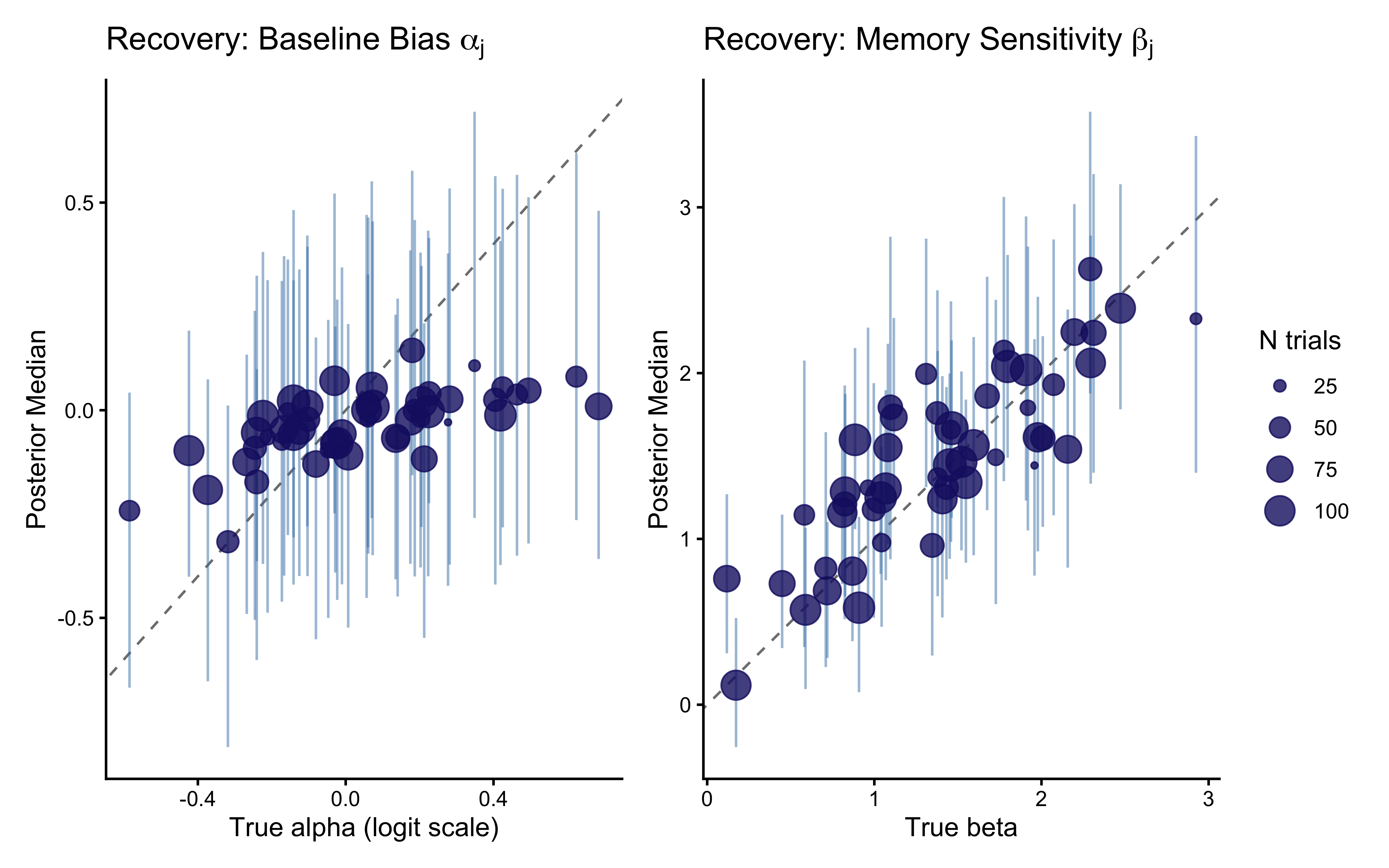

Recovery for \(\beta_j\) is typically noisier than for \(\alpha_j\) at any given trial count. The memory signal \(\text{logit}(m_{ij})\) starts at zero (the \(\text{logit}(0.5) = 0\) initialization) and becomes informative only as the cumulative opponent history diverges from 0.5. Agents with few trials show stronger shrinkage toward \(\mu_\beta = 1.5\) — not toward zero, but toward the estimated population mean, which is the appropriate regularization given what the rest of the cohort tells us about the population.

8.3.7 Prior sensitivity

sens_results_mem <- powerscale_sensitivity(
  fit_memory,
  variable = c("mu_alpha", "mu_beta", "sigma[1]", "sigma[2]", "rho")
)
cat("=== PRIOR SENSITIVITY DIAGNOSTICS: MEMORY AGENT ===\n")

## === PRIOR SENSITIVITY DIAGNOSTICS: MEMORY AGENT ===

print(sens_results_mem)

## Sensitivity based on cjs_dist
## Prior selection: all priors
## Likelihood selection: all data
## 
##  variable prior likelihood                                diagnosis
##  mu_alpha 0.058      0.027 potential strong prior / weak likelihood
##   mu_beta 0.075      0.063            potential prior-data conflict
##  sigma[1] 0.243      0.459            potential prior-data conflict
##  sigma[2] 0.437      0.202            potential prior-data conflict
##       rho 0.055      0.175            potential prior-data conflict

ps_seq_mem <- powerscale_sequence(
  fit_memory,
  variable = c("mu_alpha", "mu_beta", "sigma[1]", "sigma[2]", "rho")
)

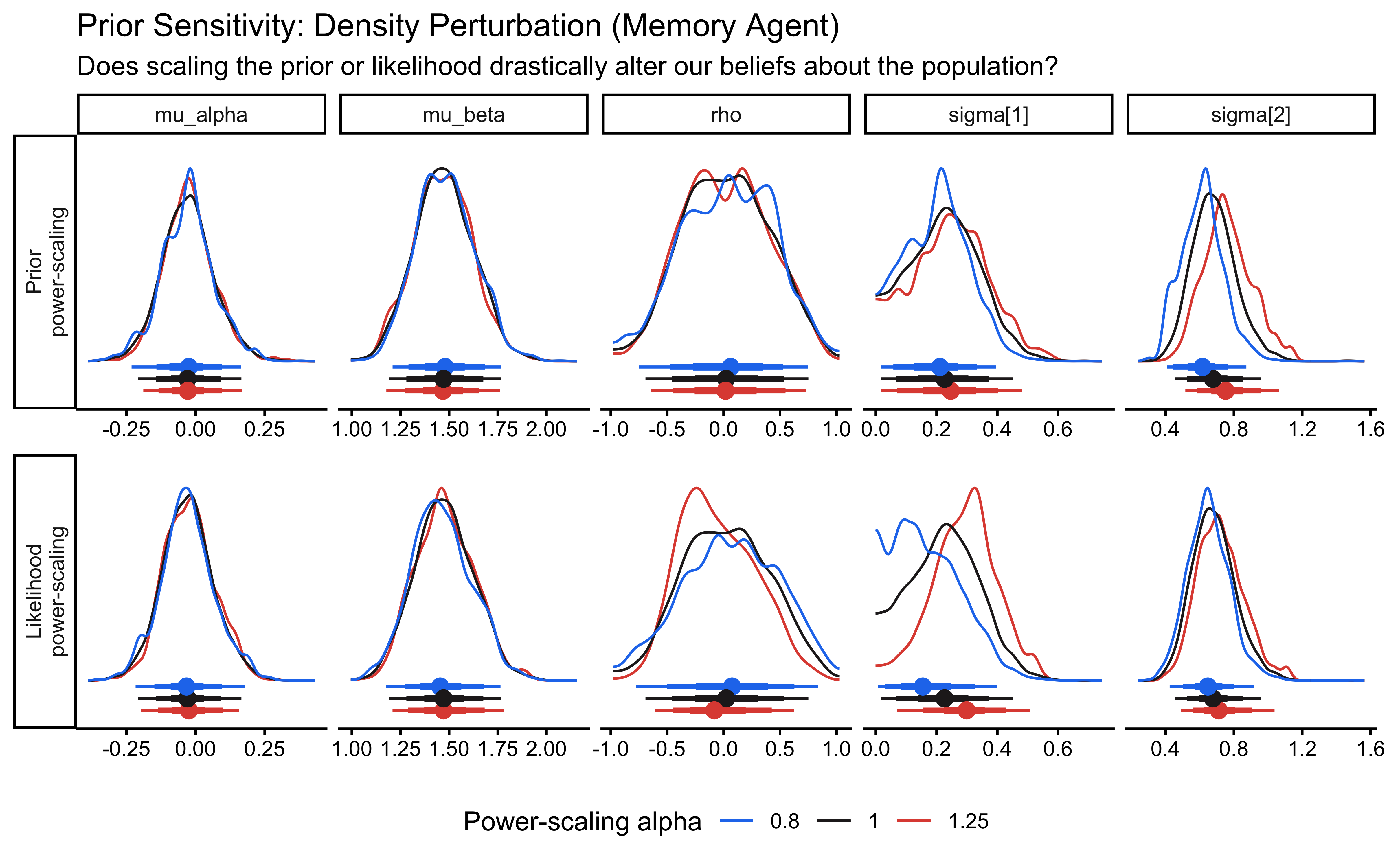
powerscale_plot_dens(ps_seq_mem) +
  labs(
    title    = "Prior Sensitivity: Density Perturbation (Memory Agent)",
    subtitle = "Does scaling the prior or likelihood drastically alter our beliefs about the population?"
  )

powerscale_plot_quantities(ps_seq_mem) +
  labs(
    title    = "Prior Sensitivity: Parameter Estimates (Memory Agent)",
    subtitle = "Horizontal lines: baseline posterior bounds. Deviations indicate sensitivity."
  )

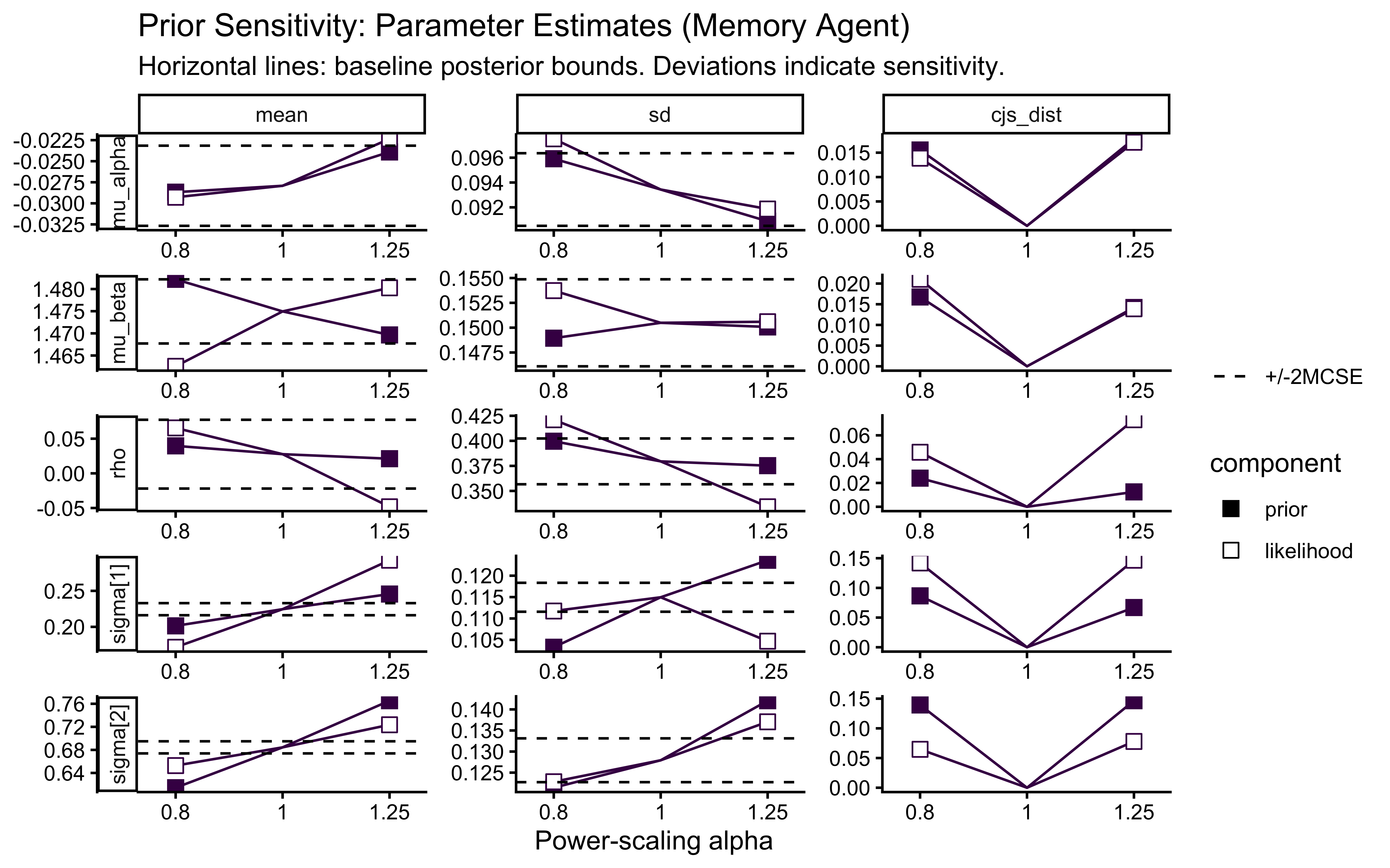
Pay particular attention to the rho panel. Because the correlation is identified only from across-agent covariation, it has fewer effective observations than the marginal population parameters. If rho shows strong sensitivity to prior scaling, the data contain limited information about the correlation structure and the LKJ prior is doing meaningful regularization.

8.3.8 Simulation-Based Calibration (SBC)

Parameter recovery on a single dataset is anecdotal. We must prove that the sampler is globally unbiased across the entire prior space.

sbc_memory_path <- here::here("simmodels", "ch6_sbc_memory.rds")

generate_sbc_dataset_memory <- function(n_agents = 50, n_trials_min = 20, n_trials_max = 120) {
  sim  <- simulate_hierarchical_memory(n_agents = n_agents,
                                        n_trials_min = n_trials_min,
                                        n_trials_max = n_trials_max)
  hp   <- attr(sim, "hyperparameters")

  list(
    variables = list(
      mu_alpha   = hp$mu_alpha,
      mu_beta    = hp$mu_beta,
      `sigma[1]` = hp$sigma_alpha,
      `sigma[2]` = hp$sigma_beta,
      rho        = hp$rho,
      alpha      = sim |> distinct(agent_id, true_alpha) |> arrange(agent_id) |> pull(true_alpha),
      beta_mem   = sim |> distinct(agent_id, true_beta)  |> arrange(agent_id) |> pull(true_beta)
    ),
    generated = prep_stan_data_memory(sim)
  )
}

generator_memory <- SBC_generator_function(
  generate_sbc_dataset_memory,
  n_agents = 50, n_trials_min = 30, n_trials_max = 120
)

backend_memory <- SBC_backend_cmdstan_sample(
  mod_memory_ncp,
  iter_warmup = 1000, iter_sampling = 1000, chains = 1, refresh = 0
)

if (regenerate_simulations || !file.exists(sbc_memory_path)) {
  sbc_datasets_memory <- generate_datasets(generator_memory, 100)
  plan(sequential)
  #future::plan(future::multisession, workers = 4)
  sbc_results_memory  <- compute_SBC(datasets = sbc_datasets_memory, backend = backend_memory,
    keep_fits = FALSE)
  saveRDS(
    list(datasets = sbc_datasets_memory, results = sbc_results_memory),
    sbc_memory_path
  )
} else {
  sbc_mem_obj         <- readRDS(sbc_memory_path)
  sbc_datasets_memory <- sbc_mem_obj$datasets
  sbc_results_memory  <- sbc_mem_obj$results
}

plot_rank_hist(sbc_results_memory, variables = c("mu_alpha", "mu_beta", "sigma[1]", "sigma[2]", "rho")) +
  labs(title = "SBC Rank Histograms: Memory Agent NCP")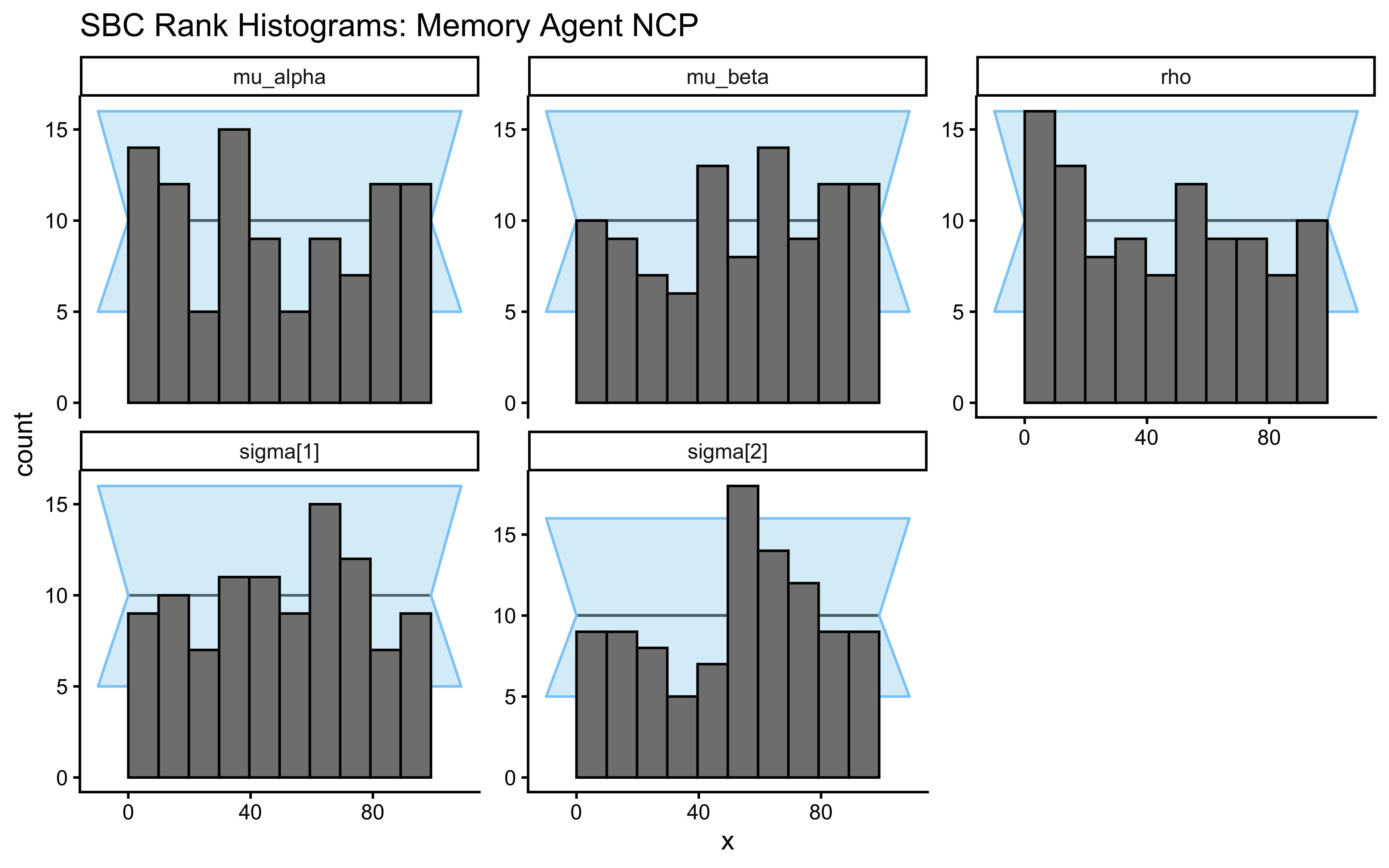

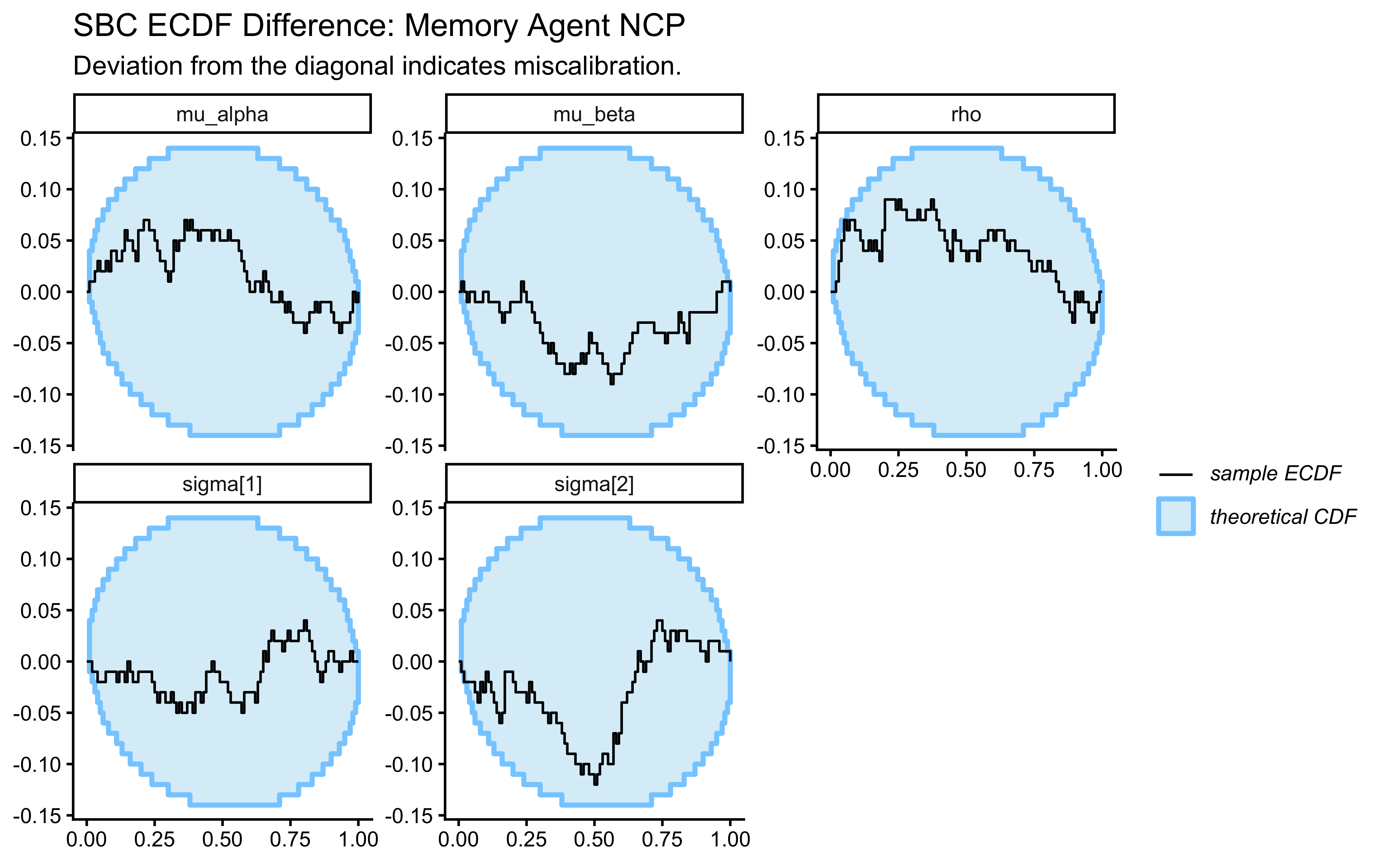
plot_ecdf_diff(sbc_results_memory, variables = c("mu_alpha", "mu_beta", "sigma[1]", "sigma[2]", "rho")) +
  labs(
    title    = "SBC ECDF Difference: Memory Agent NCP",
    subtitle = "Deviation from the diagonal indicates miscalibration."
  )

diags_memory  <- sbc_results_memory$backend_diagnostics
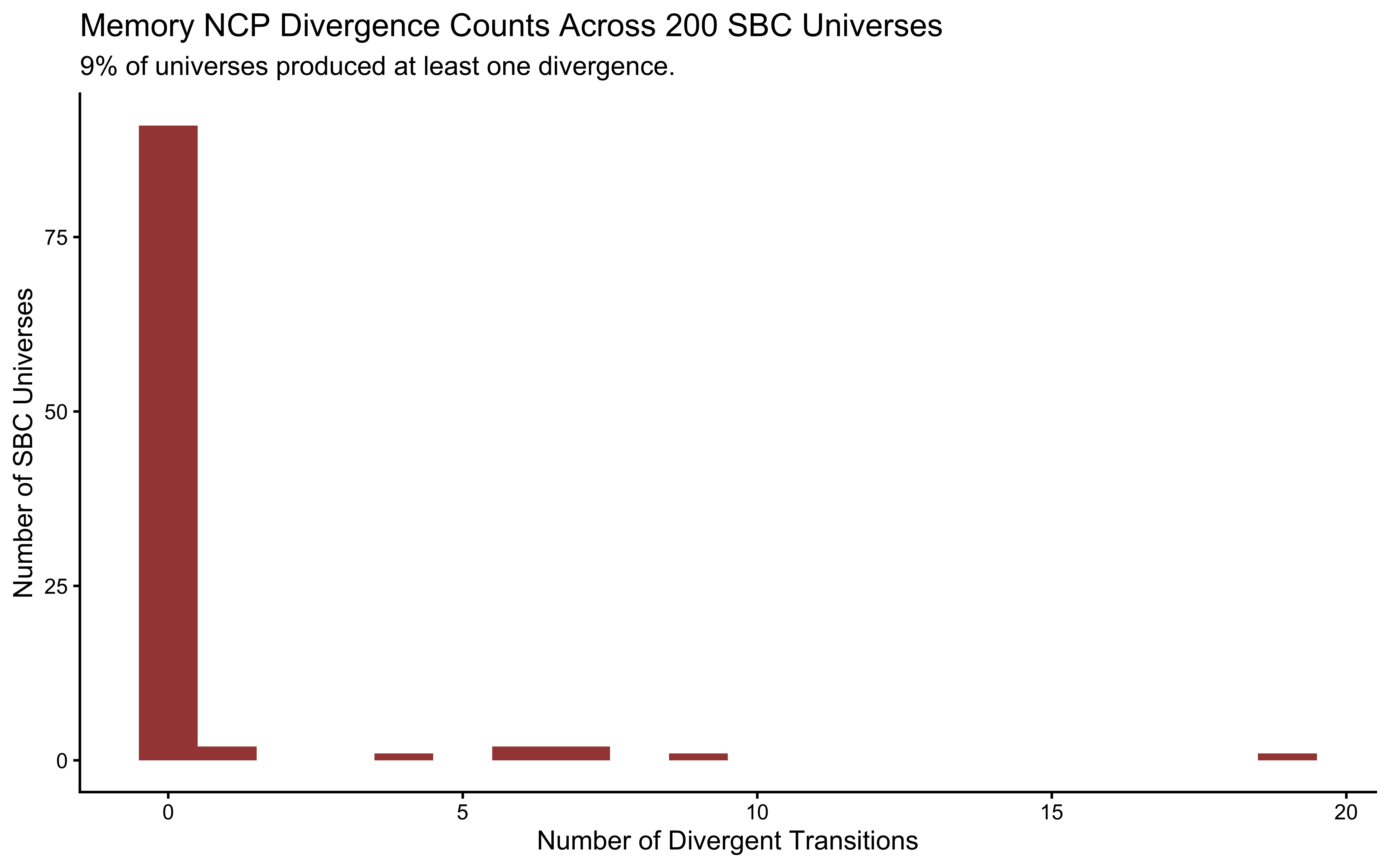
mem_fail_rate <- mean(diags_memory$n_divergent > 0) * 100

diags_memory |>
  ggplot(aes(x = n_divergent)) +
  geom_histogram(binwidth = 1, fill = "darkred", alpha = 0.8) +
  labs(
    title    = "Memory NCP Divergence Counts Across 200 SBC Universes",
    subtitle = sprintf("%.0f%% of universes produced at least one divergence.", mem_fail_rate),
    x        = "Number of Divergent Transitions",
    y        = "Number of SBC Universes"
  )

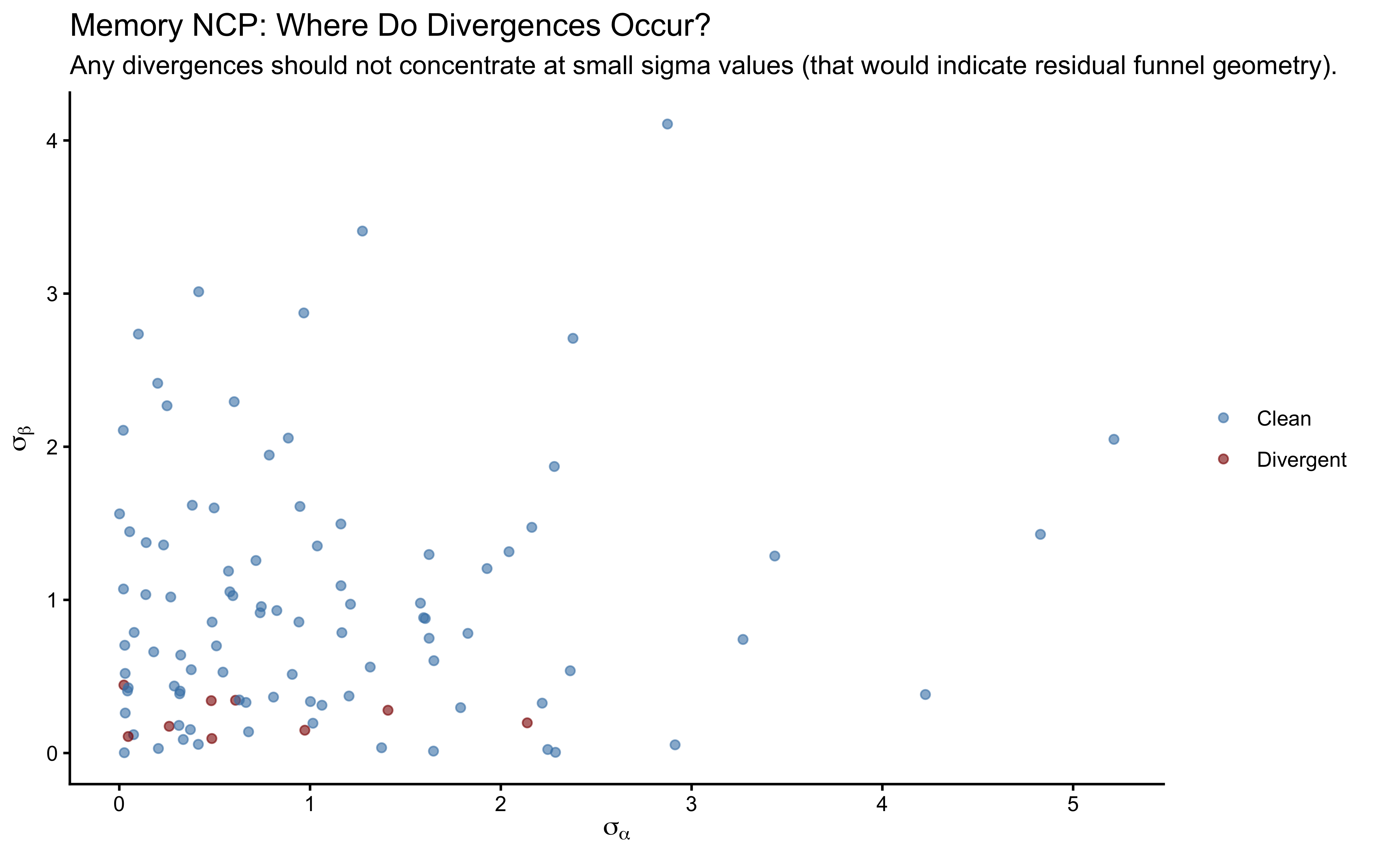
# Does any failure concentrate at small sigma values?
posterior::as_draws_df(sbc_datasets_memory$variables) |>
  as_tibble() |>
  mutate(sim_id = row_number()) |>
  left_join(
    diags_memory |> mutate(sim_id = row_number()) |> select(sim_id, n_divergent),
    by = "sim_id"
  ) |>
  mutate(had_divergence = n_divergent > 0) |>
  ggplot(aes(x = `sigma[1]`, y = `sigma[2]`, color = had_divergence)) +
  geom_point(alpha = 0.6, size = 1.5) +
  scale_color_manual(
    values = c("FALSE" = "steelblue", "TRUE" = "darkred"),
    labels = c("FALSE" = "Clean", "TRUE" = "Divergent"),
    name   = NULL
  ) +
  labs(
    title    = "Memory NCP: Where Do Divergences Occur?",
    subtitle = "Any divergences should not concentrate at small sigma values (that would indicate residual funnel geometry).",
    x        = expression(sigma[alpha]), y = expression(sigma[beta])
  )

The rho rank histogram will typically have wider confidence bands than the marginal mean and SD histograms at \(N = 200\). This is expected: \(\rho\) is identified only from covariation across \(J = 50\) agents, so each SBC universe contributes one effective draw of \(\rho\) to the calibration check. Mild irregularity within the confidence envelope is statistical noise. Systematic U-shape or strong asymmetry would indicate a genuine calibration failure.

8.3.9 Cognitive Interpretation of \(\hat{\rho}\)

The posterior on \(\rho\) is the inferential result that distinguishes this model from two independent univariate hierarchical models.

• \(\rho \approx 0\): Baseline tendency and memory-based opponent tracking are orthogonal individual differences. Studying one tells us nothing about the other.

• \(\rho > 0\): Agents with a stronger directional baseline also tend to weight memory more heavily — consistent with a general exploitation tendency, where both parameters index willingness to depart from 50/50 in response to a signal.

• \(\rho < 0\): Agents with a strong directional baseline tend to suppress memory use — a compensatory account in which prior commitment crowds out sensitivity to the opponent’s history.

None of these interpretations follow from the model alone. The model provides a calibrated posterior over \(\rho\). Cognitive theory provides the framework for deciding what that value means.

8.3.10 LOO for Model Comparison

We retain the LOO-CV score here for the model comparison section at the end of the chapter.

loo_memory <- loo(fit_memory$draws("log_lik", format = "matrix"))
print(loo_memory)

## 
## Computed from 4000 by 3774 log-likelihood matrix.
## 
##          Estimate   SE
## elpd_loo  -1965.2 29.9
## p_loo        44.8  2.3
## looic      3930.3 59.9
## ------
## MCSE of elpd_loo is NA.
## MCSE and ESS estimates assume independent draws (r_eff=1).
## 
## Pareto k diagnostic values:
##                          Count Pct.    Min. ESS
## (-Inf, 0.7]   (good)     3754  99.5%   765     
##    (0.7, 1]   (bad)        20   0.5%   <NA>    
##    (1, Inf)   (very bad)    0   0.0%   <NA>    
## See help('pareto-k-diagnostic') for details.