Chapter 2 The Pizza Experiment
📍 Where we are in the Bayesian modeling workflow: In these course notes we will introduce and consistently use a Bayesian Workflow Before we model cognition, we need to understand what modeling is — building a mechanism-based account of a system, fitting it to data, and validating it. Every move we make here (theory → math → code → fitting → checking) will repeat in every chapter that follows, now applied to minds instead of pizza stones. The full course roadmap is in the section below.
2.1 From Pizza to Cognitive Models: An Introduction
This chapter introduces core modeling concepts through a delicious lens: the physics of pizza stone heating. While this might seem far removed from cognitive science, it provides an insightful introduction to the challenges and methodologies of modeling complex phenomena.
2.2 Why Start with Pizza?
Do I even need to answer that question? Because pizza, obviously.
Beyond the universal appeal of pizza, starting with a physical system like a heating pizza stone offers a tangible way to grasp core principles fundamental to cognitive modeling. Understanding human cognition involves tackling immense complexity – often dealing with hidden mental states, noisy behavioral data, and competing theories. Modeling a pizza stone allows us to isolate and understand key methodological challenges in a more constrained environment.
First, it demonstrates how to bridge theory and math. We rely on Prior Knowledge — using Newton’s Law of Cooling to structure our equations — just as cognitive scientists use theories of memory or attention to guide their models. This forces us to critically determine our Levels of Analysis: just as we simplify complex thermodynamics into a basic cooling formula, cognitive scientists must decide whether to model neurons, beliefs, or behavioral choices.
It also highlights the problem of Latent Variables. Just as we cannot “see” a heating coefficient—only the noisy temperatures it produces—we cannot see a “learning rate” in the brain, only the choices it drives.
Finally, this example acts as a sandbox for Model Complexity and Validation. We will explicitly compare detailed physics-based models against simpler statistical approximations to see which performs better on empirical data. This mirrors the central trade-off in cognitive science: balancing theoretical completeness with the practical utility of generating testable predictions from available data.
2.3 Learning Objectives
This chapter uses the seemingly simple example of a heating pizza stone to introduce fundamental principles of computational modeling that are directly applicable to cognitive science. While the specific physics and code are illustrative, the core goals are to understand the process of modeling.
By completing this chapter, you will be able to:
Appreciate Generative Modeling: Understand the value of building models based on underlying mechanisms (like physics or cognitive processes) rather than just describing data patterns.
Connect Theory and Data: See how theoretical knowledge (physics laws) informs model structure and how data is used to estimate unknown model parameters (like the heating coefficient).
Implement and Fit Models: Gain initial experience implementing mathematical models in code (R and Stan) and using Bayesian inference (
brms,cmdstanr) to fit them to empirical data.Evaluate Model Fit: Learn basic techniques for visualizing model predictions against data and understand the limitations of purely statistical models compared to theory-driven ones.
Recognize Modeling Trade-offs: Understand the balance between model complexity, theoretical grounding, and practical utility through comparing statistical vs. physics-based approaches.
Apply Modeling Principles: Recognize how the steps taken here – data exploration, model building, parameter estimation, validation – form a general workflow applicable to cognitive modeling problems explored later in the course.
Oh, and you’ll probably get hungry as well!
Required Packages
# 1. Ensure 'pacman' is installed
if (!require("pacman")) install.packages("pacman")

# 2. Load packages (pacman will verify, install if missing, and load them)
pacman::p_load(
  tidyverse,  # Core package for data manipulation and visualization
  brms,       # Interface for Bayesian regression models using Stan
  bayesplot,  # Convenient functions for plotting Bayesian model results
  tidybayes,  # Utilities for working with Bayesian model outputs in a tidy format
  cmdstanr,    # Backend interface for running Stan models efficiently
  here        # For constructing file paths relative to project root
)
2.4 Part 1: Exploring the Pizza Stone Temperature Data
In this study, we collected temperature measurements from a pizza stone in a gas-fired oven using an infrared temperature gun. Three different raters (N, TR, and R) took measurements over time to track how the stone heated up. Understanding how pizza stones heat up is crucial for achieving the perfect pizza crust, as consistent and sufficient stone temperature is essential for proper baking.
The measurements were taken as follows:
# Load and examine the data
data <- tibble(
  Order = rep(0:18, 3),
  Seconds = rep(c(0, 175, 278, 333, 443, 568, 731, 773, 851, 912, 980,
                  1040, 1074, 1124, 1175, 1237, 1298, 1359, 1394), 3),
  Temperature = c(15.1, 233, 244, 280, 289, 304, 343, NA, 333, 341, 320,
                  370, 325, 362, 363, 357, 380, 376, 380,
                  14.5, 139.9, 153, 36.1, 254, 459, 263, 369, rep(NA, 11),
                  12.9, 149.5, 159, 179.4, 191.7, 201, 210, NA, 256, 257,
                  281, 293, 297, 309, 318, 321, rep(NA, 3)),
  Rater = rep(c("N", "TR", "R"), each = 19)
)


# Create summary statistics
summary_stats <- data %>%
  group_by(Rater) %>%
  summarize(
    n_measurements = sum(!is.na(Temperature)),
    mean_temp = mean(Temperature, na.rm = TRUE),
    sd_temp = sd(Temperature, na.rm = TRUE),
    min_temp = min(Temperature, na.rm = TRUE),
    max_temp = max(Temperature, na.rm = TRUE)
  )

# Display summary statistics
knitr::kable(summary_stats, digits = 1)| Rater | n_measurements | mean_temp | sd_temp | min_temp | max_temp |
|---|---|---|---|---|---|
| N | 18 | 312.0 | 86.4 | 15.1 | 380 |
| R | 15 | 229.0 | 83.9 | 12.9 | 321 |
| TR | 8 | 211.1 | 155.2 | 14.5 | 459 |
2.4.1 Initial Data Visualization
Let’s visualize how the temperature evolves over time for each rater:
ggplot(data, aes(x = Seconds/60, y = Temperature, color = Rater)) +
  geom_point(size = 3, alpha = 0.7) +
  geom_line(alpha = 0.5) +
  labs(
    title = "Pizza Stone Temperature Evolution",
    subtitle = "Measurements by three different raters",
    x = "Time (minutes)",
    y = "Temperature (°C)",
    color = "Rater"
  ) +
  theme_bw() +
  scale_color_brewer(palette = "Set1")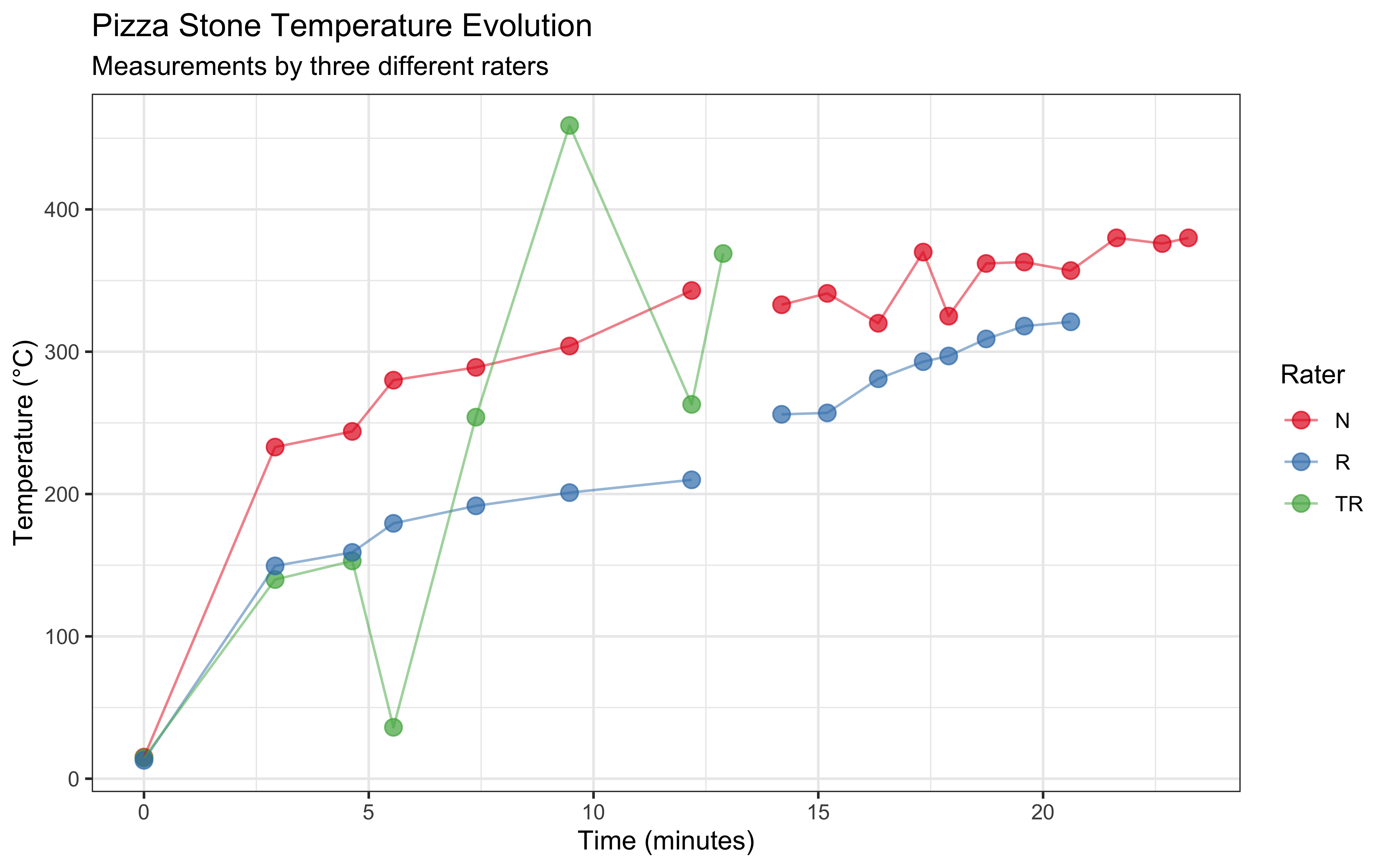
2.4.2 Key Observations
Several interesting patterns emerge from our data:
Heating Patterns: The temperature generally increases over time, but not uniformly. We observe some fluctuations that might be due to:
- Variation in gas flame intensity
- Different measurement locations on the stone
- Measurement technique differences between raters
Measurement Patterns by Rater
- Rater N maintained consistent measurements throughout the experiment
- Rater TR shows more variability and fewer total measurements
- Rater R shows a more gradual temperature increase pattern
Missing Data: Some measurements are missing (NA values), particularly in the later time points for Rater TR. This is common in real-world data collection and needs to be considered in our analysis.
Let’s examine the rate of temperature change:
# --- Calculate Rate of Temperature Change ---
# To understand how quickly the stone heats up, calculate the change rate per minute.
data_with_rate <- data %>%
  group_by(Rater) %>% # Perform calculation separately for each rater
  arrange(Seconds) %>% # Ensure data is sorted chronologically for lag function
  mutate(
    # Calculate difference in temperature from previous measurement
    delta_temp = Temperature - lag(Temperature),
    # Calculate time elapsed since previous measurement
    delta_secs = Seconds - lag(Seconds),
    # Calculate rate in degrees C per second, then convert to degrees C per minute
    temp_change_per_min = (delta_temp / delta_secs) * 60,
    # Convert time to minutes for plotting
    minutes = Seconds / 60
  ) %>%
  # Remove rows where rate couldn't be calculated (i.e., the first row for each rater)
  filter(!is.na(temp_change_per_min))

# Visualize temperature change rate
ggplot(data_with_rate, aes(x = minutes, y = temp_change_per_min, color = Rater)) +
  geom_point() +
  geom_line() +
  labs(
    title = "Rate of Temperature Change Over Time",
    subtitle = "Degrees Celsius per minute",
    x = "Time (minutes)",
    y = "Temperature Change Rate (°C/min)",
    color = "Rater"
  ) +
  theme_bw() +
  scale_color_brewer(palette = "Set1")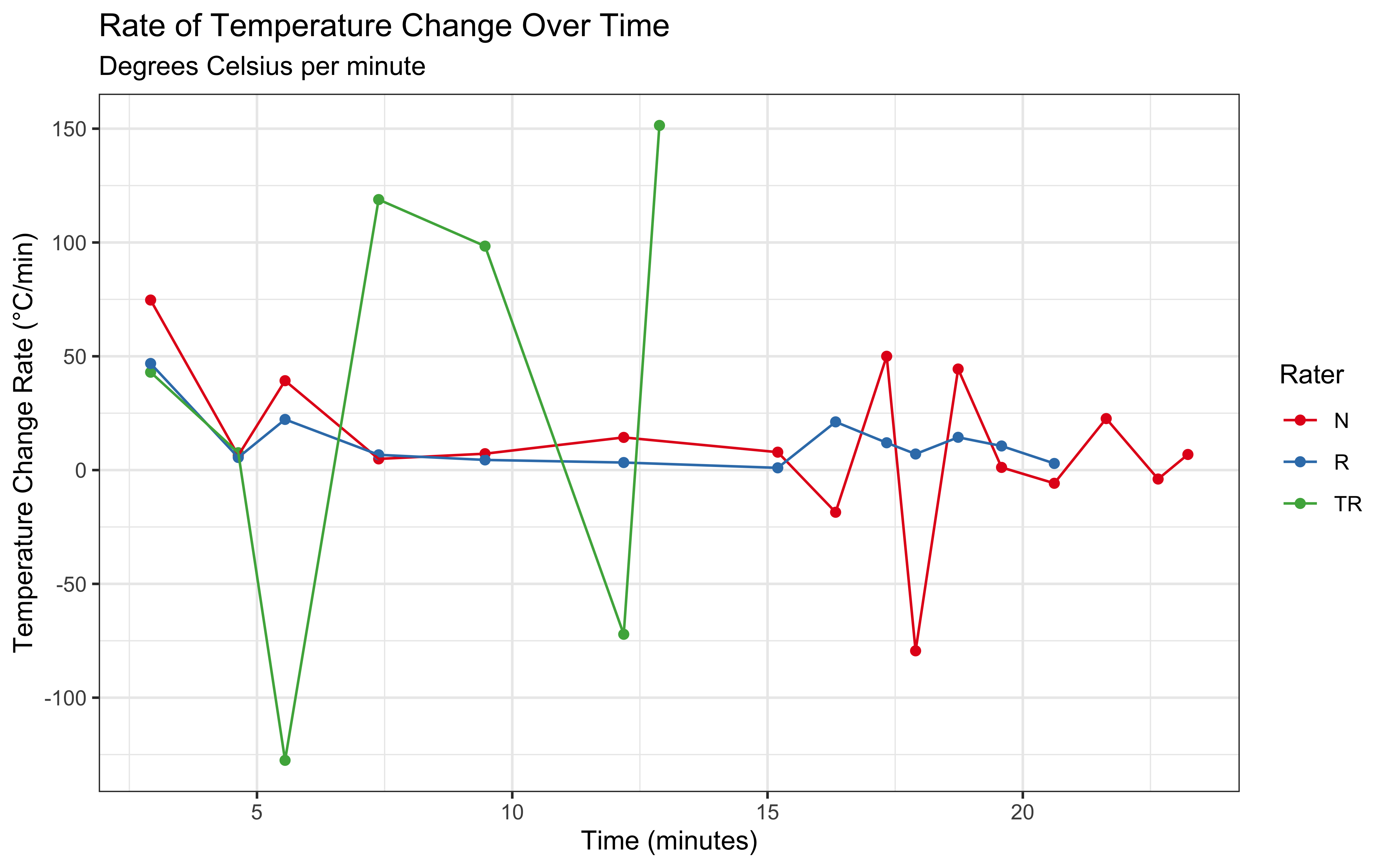
This visualization reveals that the heating rate is (likely) highest in the first few minutes and gradually decreases as the stone temperature approaches the oven temperature. This aligns with Newton’s Law of Cooling/Heating, which we will explore in the next section.
2.5 Part 2: Initial Statistical Modeling
Before developing our physics-based model, let’s explore how standard statistical approaches perform in modeling our temperature data. We’ll implement two types of models using the brms package: a linear mixed-effects model and a lognormal mixed-effects model. Both models will account for variations between raters.
2.5.1 Model Setup and Priors
First, let’s ensure we have a directory for our models and set up our computational parameters:
# --- Model Fitting Setup ---
# Define relative paths for saving model objects and Stan code.
linear_model_path <- here("models", "01_pizza_linear_model")
lognormal_model_path <- here("models", "01_pizza_lognormal_model")
stan_model_path <- here("models", "pizza_physics_model.stan")

# Create the 'models' directory if it doesn't already exist
if (!dir.exists("models")) {
  dir.create("models")
  message("Created 'models' directory.")
}

# Define computational parameters
mc_settings <- list(
  chains = 2,
  iter = 6000,
  seed = 123,
  backend = "cmdstanr"
)
2.5.2 Linear Mixed-Effects Model
We begin with a linear mixed-effects model, which assumes that temperature increases linearly with time but allows for different patterns across raters. This model includes both fixed effects (overall time trend) and random effects (rater-specific variations).
data_scaled <- data %>%
  mutate(Minutes = Seconds / 60)

# Define priors for linear model
linear_priors <- c(
  prior(normal(15, 20), class = "Intercept"),  # Centered around room temperature
  prior(normal(0, 20), class = "b"),          # Expected temperature change per minute
  prior(normal(0, 50), class = "sigma"),         # Residual variation
  prior(normal(0, 50), class = "sd"),            # Random effects variation
  prior(lkj(3), class = "cor")                    # Random effects correlation
)

# --- Linear Model ---
linear_model <- brm(
  Temperature ~ Minutes + (1 + Minutes | Rater),
  data = data_scaled,
  family = gaussian,
  prior = linear_priors,
  chains = mc_settings$chains,
  iter = mc_settings$iter,
  seed = mc_settings$seed, # Ensures reproducibility of MCMC sampling
  backend = mc_settings$backend,
  file = linear_model_path, # Use relative path
  file_refit = "on_change", # Refit if model code or data changes
  cores = 2, # Specify cores used for parallel chains
  # Increased adapt_delta and max_treedepth help prevent divergent transitions
  adapt_delta = 0.99,
  max_treedepth = 20
)

# Display model summary
summary(linear_model)
## Family: gaussian
## Links: mu = identity
## Formula: Temperature ~ Minutes + (1 + Minutes | Rater)
## Data: data_scaled (Number of observations: 41)
## Draws: 2 chains, each with iter = 6000; warmup = 3000; thin = 1;
## total post-warmup draws = 6000
##
## Multilevel Hyperparameters:
## ~Rater (Number of levels: 3)
## Estimate Est.Error l-95% CI u-95% CI Rhat Bulk_ESS Tail_ESS
## sd(Intercept) 57.01 28.21 7.42 120.86 1.00 2014 1104
## sd(Minutes) 31.39 15.76 11.83 71.91 1.00 1655 2789
## cor(Intercept,Minutes) 0.00 0.35 -0.65 0.65 1.00 2075 3209
##
## Regression Coefficients:
## Estimate Est.Error l-95% CI u-95% CI Rhat Bulk_ESS Tail_ESS
## Intercept 84.92 45.64 -13.93 166.45 1.00 1809 2567
## Minutes -5.54 4.21 -13.23 3.41 1.00 1816 2506
##
## Further Distributional Parameters:
## Estimate Est.Error l-95% CI u-95% CI Rhat Bulk_ESS Tail_ESS
## sigma 57.45 6.87 45.63 72.47 1.00 3734 3283
##
## Draws were sampled using sample(hmc). For each parameter, Bulk_ESS
## and Tail_ESS are effective sample size measures, and Rhat is the potential
## scale reduction factor on split chains (at convergence, Rhat = 1).2.5.3 Lognormal Mixed-Effects Model
The lognormal model accounts for the fact that temperature changes might be proportional rather than additive, and ensures predictions cannot go below zero (I don’t bring my oven out in the freezing cold!).
# Define priors for lognormal model
lognormal_priors <- c(
  prior(normal(2.7, 0.5), class = "Intercept"),     # Log scale for room temperature
  prior(normal(0, 0.3), class = "b"),     # Expected log-scale change per minute
  prior(normal(0, 1), class = "sigma"),        # Log-scale residual variation
  prior(normal(0, 0.5), class = "sd"),           # Random effects variation
  prior(lkj(3), class = "cor")                   # Random effects correlation
)

# --- Lognormal Model ---
lognormal_model <- brm(
  Temperature ~ Minutes + (1 + Minutes | Rater),
  data = data_scaled,
  family = lognormal, # Use lognormal distribution
  prior = lognormal_priors,
  chains = mc_settings$chains,
  cores = 2,
  adapt_delta = 0.99,
  max_treedepth = 20,
  iter = mc_settings$iter,
  seed = mc_settings$seed, # Use the same seed for comparison if desired
  backend = mc_settings$backend,
  file = lognormal_model_path, # Use relative path
  file_refit = "on_change"
)

# Generate predictions
lognormal_preds <- fitted(
  lognormal_model,
  newdata = data_scaled,
  probs = c(0.025, 0.975)
) %>%
  as_tibble() %>%
  bind_cols(data)
2.5.4 Model Comparison and Visualization
Let’s compare how these models fit our data:
# Compare models using LOO
model_comparison <- loo_compare(
  loo(linear_model),
  loo(lognormal_model)
)

# Create comparison plot
ggplot() +
  # Raw data points
  geom_point(data = data,
            aes(x = Seconds/60, y = Temperature, color = Rater),
            alpha = 0.5) +
  # Linear model predictions
  geom_line(data = linear_preds,
            aes(x = Seconds/60, y = Estimate, linetype = "Linear"),
            color = "blue") +
  geom_ribbon(data = linear_preds,
              aes(x = Seconds/60, ymin = Q2.5, ymax = Q97.5),
              fill = "blue", alpha = 0.1) +
  # Lognormal model predictions
  geom_line(data = lognormal_preds,
            aes(x = Seconds/60, y = Estimate, linetype = "Lognormal"),
            color = "red") +
  geom_ribbon(data = lognormal_preds,
              aes(x = Seconds/60, ymin = Q2.5, ymax = Q97.5),
              fill = "red", alpha = 0.1) +
  # Formatting
  facet_wrap(~Rater) +
  labs(
    title = "Comparison of Statistical Models",
    subtitle = "Linear vs Lognormal Mixed-Effects Models",
    x = "Time (minutes)",
    y = "Temperature (°C)",
    linetype = "Model Type"
  ) +
  theme_bw()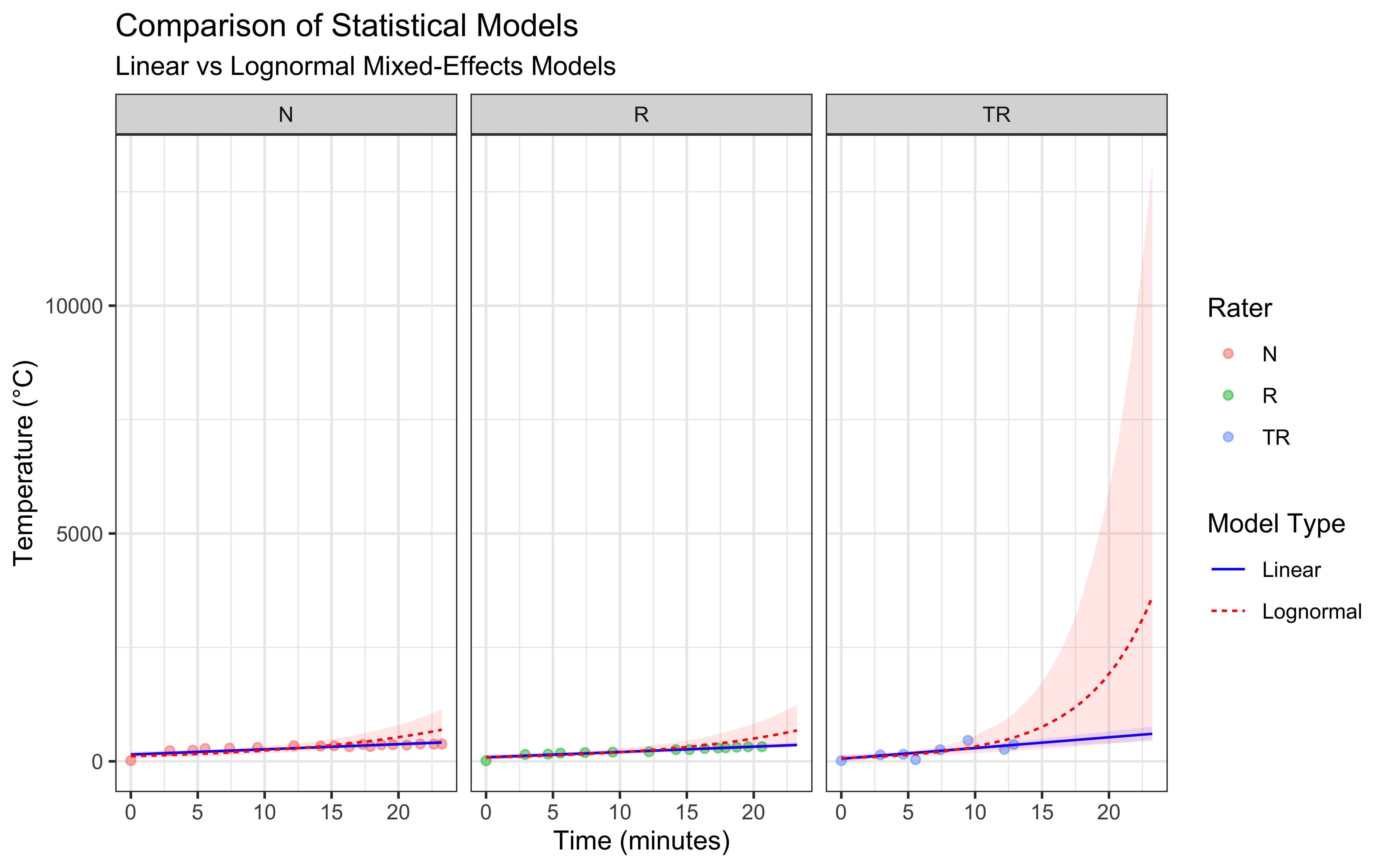
# Create comparison plot but capping the y axis
ggplot() +
  # Raw data points
  geom_point(data = data,
            aes(x = Seconds/60, y = Temperature, color = Rater),
            alpha = 0.5) +
  # Linear model predictions
  geom_line(data = linear_preds,
            aes(x = Seconds/60, y = Estimate, linetype = "Linear"),
            color = "blue") +
  geom_ribbon(data = linear_preds,
              aes(x = Seconds/60, ymin = Q2.5, ymax = Q97.5),
              fill = "blue", alpha = 0.1) +
  # Lognormal model predictions
  geom_line(data = lognormal_preds,
            aes(x = Seconds/60, y = Estimate, linetype = "Lognormal"),
            color = "red") +
  geom_ribbon(data = lognormal_preds,
              aes(x = Seconds/60, ymin = Q2.5, ymax = Q97.5),
              fill = "red", alpha = 0.1) +
  ylim(0, 1000) +
  # Formatting
  facet_wrap(~Rater) +
  labs(
    title = "Comparison of Statistical Models",
    subtitle = "Linear vs Lognormal Mixed-Effects Models",
    x = "Time (minutes)",
    y = "Temperature (°C)",
    linetype = "Model Type"
  ) +
  theme_bw()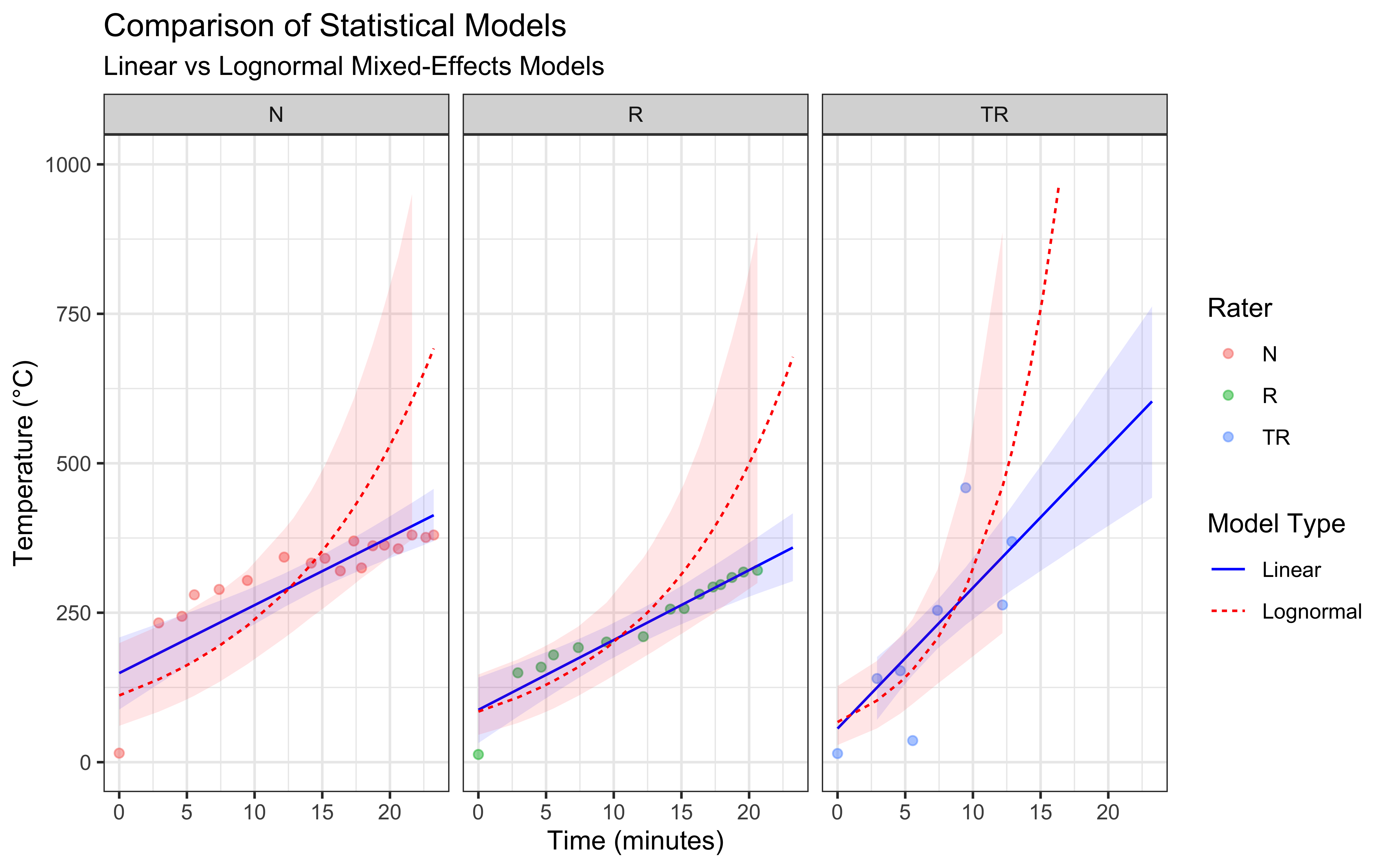
2.5.5 Model Assessment
I have seen worse models in my time, but they do seem to have important issues:
The linear mixed-effects model assumes a constant rate of temperature change, which we can see is not at all accurate. The actual temperature increase is fast at the beginning and appears to slow down over time, particularly at higher temperatures. While this model has the advantage of simplicity, it is not likely to produce accurate predictions as it seem to fail to capture the underlying physics of heat transfer.
The lognormal mixed-effects model is completely off.
Further, the lognormal model produce some divergences. In a Bayesian workflow, divergences indicate that the Hamiltonian Monte Carlo sampler is exploring pathological posterior geometry. Because purely statistical models lack mechanistic asymptotes, they explore parameter spaces that lead to mathematically unstable extrapolations. The core issue is that neither model incorporates our knowledge of heat transfer physics: e.g the flame temperature limiting the temperature the stone can reach and the exponential approach to equilibrium temperature. This limitation motivates our next section, where we’ll develop a physics-based model.
2.6 Part 3: Understanding the Physics Model
Temperature evolution in a pizza stone follows Newton’s Law of Cooling/Heating. We’ll start by exploring this physical model before applying it to real data.
2.6.1 The Basic Temperature Evolution Equation
The temperature evolution of a pizza stone in a gas-fired oven is governed by the heat diffusion equation, which describes how heat flows through solid materials:
\[\rho c_p \frac{\partial T}{\partial t} = k\nabla^2T + Q\]
where: \(\rho\) represents the stone’s density (kg/m³) \(c_p\) denotes specific heat capacity (J/kg·K) \(T\) is temperature (K) \(t\) represents time (s) \(k\) is thermal conductivity (W/m·K) \(\nabla^2\) is the Laplacian operator \(Q\) represents heat input from the oven (W/m³)
While this equation provides a complete description of heat flow, we can significantly simplify our analysis by applying the lumped capacitance model. his simplification assumes that the stone conducts heat internally much faster than it absorbs it from the surface. This allows us to ignore the complex internal gradients (\(\nabla^2T\)) and focus purely on the surface heat transfer, reducing our model to:
\[\frac{dT}{dt} = \frac{hA}{mc_p}(T_{\infty} - T)\]
where: \(h\) is the heat transfer coefficient (W/m²·K) \(A\) is the surface area exposed to heat (m²) \(m\) is the stone’s mass (kg) \(T_{\infty}\) is the oven temperature (K)
This simplified equation relates the rate of temperature change to the difference between the current stone temperature T and the ambient temperature T∞ (as determined by the flame). The coefficient h represents the heat transfer coefficient between the ambient and stone, A is the stone’s surface area exposed to heat, m is its mass, and cp remains the specific heat capacity.
To solve this differential equation, we begin by separating variables:
\[\frac{dT}{T_{\infty} - T} = \left(\frac{hA}{mc_p}\right)dt\]
Integration of both sides yields:
\[-\ln|T_{\infty} - T| = \left(\frac{hA}{mc_p}\right)t + C\]
where C is an integration constant.
Using the initial condition \(T = T_i\) at \(t = 0\), we can determine the integration constant:
\[C = -\ln|T_{\infty} - T_i|\]
Substituting this back and solving for temperature gives us:
\[T = T_{\infty} + (T_i - T_{\infty})\exp\left(-\frac{hA}{mc_p}t\right)\]
For practical reasons, we combine physical parameters into a single coefficient, which we will call HOT:
\[HOT = \frac{hA}{mc_p}\] Giving our working equation: \[T = T_{\infty} + (T_i - T_{\infty})\exp(-HOT \cdot t)\]
This equation retains the essential physics while providing a practical model for analyzing our experimental data. The HOT coefficient encapsulates the combined effects of heat transfer efficiency, stone geometry, and material properties into a single parameter that determines how quickly the stone approaches the flame temperature.
2.7 Part 4: Implementing the Physics-Based Model
Having established the theoretical foundation, we now face a practical challenge: we cannot measure \(h\), \(A\), or \(c_p\) directly during the bake. Instead, we must infer the aggregate parameter HOT from the noisy temperature data collected by our raters. This is where Stan comes in, enabling us to create a Bayesian implementation of our physics-based model, and to account for measurement uncertainty and variation between raters. First, we prepare our data for the Stan model. Our model requires initial temperatures, time measurements, and observed temperatures from each rater:
# Create data structure for Stan
stan_data <- list(
  N = nrow(data %>% filter(!is.na(Temperature))),
  time = data %>% filter(!is.na(Temperature)) %>% pull(Seconds),
  temp = data %>% filter(!is.na(Temperature)) %>% pull(Temperature),
  n_raters = 3,
  rater = as.numeric(factor(data %>%
                           filter(!is.na(Temperature)) %>%
                           pull(Rater))),
  Ti = c(15.1, 14.5, 12.9),  # Initial temperature estimates
  Tinf = 450              # Flame temperature estimate
)
Next, we implement our physics-based model in Stan. The model incorporates our derived equation while allowing for rater-specific heating coefficients:
stan_code <- "
data {
  int<lower=0> N;                   // Number of observations
  vector[N] time;                   // Time points
  vector[N] temp;                   // Observed temperatures
  int<lower=0> n_raters;           // Number of raters
  array[N] int<lower=1,upper=n_raters> rater;  // Rater indices
  vector[n_raters] Ti;             // Initial temperatures
  real Tinf;                       // Flame temperature
}

parameters {
  vector<lower=0>[n_raters] HOT;   // Heating coefficients
  vector<lower=0>[n_raters] sigma; // Measurement error
}

model {
  // Physics-based temperature prediction
  vector[N] mu = Tinf + (Ti[rater] - Tinf) .* exp(-HOT[rater] .* time);

  // Prior distributions
  target += normal_lpdf(HOT | 0.005, 0.005);    // Prior for heating rate
  target += exponential_lpdf(sigma | 1);         // Prior for measurement error

  // Likelihood
  target += normal_lpdf(temp | mu, sigma[rater]);
}
"

# Save the Stan model code using the relative path
writeLines(stan_code, stan_model_path)

# Compile and fit the Stan model using the relative path
# Compilation happens once; subsequent runs load the compiled object if unchanged.
mod <- cmdstan_model("models/pizza_physics_model.stan")
2.7.1 Prior Predictive Check
Before fitting our model to empirical data, we must ensure our priors generate physically plausible heating curves (Simulation Validation). If our normal(0.005, 0.005) prior on HOT is appropriate, simulated temperatures should gradually approach \(T_{\infty}\) without exceeding it or dropping below absolute zero.
# Simulate HOT parameters from the prior
set.seed(123)
prior_hot <- rnorm(100, mean = 0.005, sd = 0.005)
prior_hot <- prior_hot[prior_hot > 0] # Truncate at 0 as per Stan lower=0 bound

# Simulate curves
time_seq <- seq(0, max(stan_data$time), length.out = 100)
prior_preds <- expand_grid(sim_id = 1:length(prior_hot), time = time_seq) %>%
  mutate(
    hot = prior_hot[sim_id],
    temp = stan_data$Tinf + (15.0 - stan_data$Tinf) * exp(-hot * time)
  )

ggplot(prior_preds, aes(x = time/60, y = temp, group = sim_id)) +
  geom_line(alpha = 0.2, color = "blue") +
  labs(title = "Prior Predictive Check: Heating Curves",
       x = "Time (minutes)", y = "Temperature (°C)") +
  theme_bw()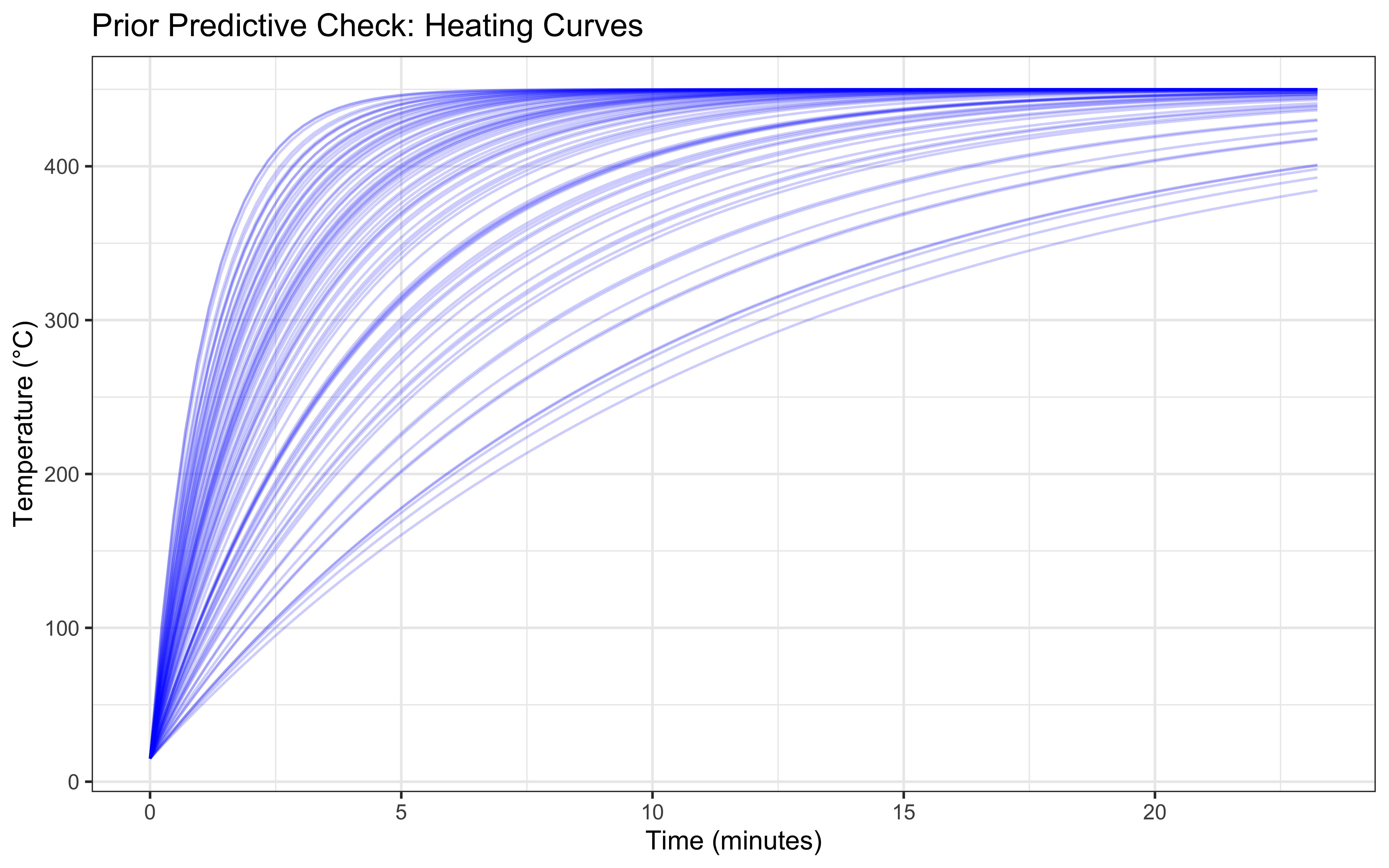
## Running MCMC with 2 parallel chains...
##
## Chain 1 Iteration:    1 / 2000 [  0%]  (Warmup)
## Chain 1 Iteration:  100 / 2000 [  5%]  (Warmup)
## Chain 1 Iteration:  200 / 2000 [ 10%]  (Warmup)
## Chain 1 Iteration:  300 / 2000 [ 15%]  (Warmup)
## Chain 1 Iteration:  400 / 2000 [ 20%]  (Warmup)
## Chain 1 Iteration:  500 / 2000 [ 25%]  (Warmup)
## Chain 1 Iteration:  600 / 2000 [ 30%]  (Warmup)
## Chain 1 Iteration:  700 / 2000 [ 35%]  (Warmup)
## Chain 1 Iteration:  800 / 2000 [ 40%]  (Warmup)
## Chain 1 Iteration:  900 / 2000 [ 45%]  (Warmup)
## Chain 1 Iteration: 1000 / 2000 [ 50%]  (Warmup)
## Chain 1 Iteration: 1001 / 2000 [ 50%]  (Sampling)
## Chain 1 Iteration: 1100 / 2000 [ 55%]  (Sampling)
## Chain 1 Iteration: 1200 / 2000 [ 60%]  (Sampling)
## Chain 1 Iteration: 1300 / 2000 [ 65%]  (Sampling)
## Chain 1 Iteration: 1400 / 2000 [ 70%]  (Sampling)
## Chain 1 Iteration: 1500 / 2000 [ 75%]  (Sampling)
## Chain 1 Iteration: 1600 / 2000 [ 80%]  (Sampling)
## Chain 1 Iteration: 1700 / 2000 [ 85%]  (Sampling)
## Chain 1 Iteration: 1800 / 2000 [ 90%]  (Sampling)
## Chain 1 Iteration: 1900 / 2000 [ 95%]  (Sampling)
## Chain 1 Iteration: 2000 / 2000 [100%]  (Sampling)
## Chain 2 Iteration:    1 / 2000 [  0%]  (Warmup)
## Chain 2 Iteration:  100 / 2000 [  5%]  (Warmup)
## Chain 2 Iteration:  200 / 2000 [ 10%]  (Warmup)
## Chain 2 Iteration:  300 / 2000 [ 15%]  (Warmup)
## Chain 2 Iteration:  400 / 2000 [ 20%]  (Warmup)
## Chain 2 Iteration:  500 / 2000 [ 25%]  (Warmup)
## Chain 2 Iteration:  600 / 2000 [ 30%]  (Warmup)
## Chain 2 Iteration:  700 / 2000 [ 35%]  (Warmup)
## Chain 2 Iteration:  800 / 2000 [ 40%]  (Warmup)
## Chain 2 Iteration:  900 / 2000 [ 45%]  (Warmup)
## Chain 2 Iteration: 1000 / 2000 [ 50%]  (Warmup)
## Chain 2 Iteration: 1001 / 2000 [ 50%]  (Sampling)
## Chain 2 Iteration: 1100 / 2000 [ 55%]  (Sampling)
## Chain 2 Iteration: 1200 / 2000 [ 60%]  (Sampling)
## Chain 2 Iteration: 1300 / 2000 [ 65%]  (Sampling)
## Chain 2 Iteration: 1400 / 2000 [ 70%]  (Sampling)
## Chain 2 Iteration: 1500 / 2000 [ 75%]  (Sampling)
## Chain 2 Iteration: 1600 / 2000 [ 80%]  (Sampling)
## Chain 2 Iteration: 1700 / 2000 [ 85%]  (Sampling)
## Chain 2 Iteration: 1800 / 2000 [ 90%]  (Sampling)
## Chain 2 Iteration: 1900 / 2000 [ 95%]  (Sampling)
## Chain 2 Iteration: 2000 / 2000 [100%]  (Sampling)
## Chain 1 finished in 0.1 seconds.
## Chain 2 finished in 0.1 seconds.
##
## Both chains finished successfully.
## Mean chain execution time: 0.1 seconds.
## Total execution time: 1.7 seconds.
The Stan implementation translates our mathematical model into a computational framework. We assign informative priors to our parameters based on physical understanding: the heating coefficient (HOT) is expected to be small but positive, while measurement error (sigma) follows an exponential distribution to ensure positivity while allowing for varying levels of uncertainty between raters. To visualize our model’s predictions and assess its performance, we extract posterior samples and generate predictions across our time range:
# Extract draws
post <- as_draws_df(fit$draws()) %>%
  dplyr::select(starts_with("HOT"), starts_with("sigma")) %>%
  slice_sample(n = 100)

# Create prediction grid
pred_data <- tidyr::crossing(
  time = seq(0, max(stan_data$time), length.out = 100),
  rater = 1:stan_data$n_raters
) %>%
  mutate(
    Ti = stan_data$Ti[rater],
    Tinf = stan_data$Tinf
  )

# Generate predictions
pred_matrix <- matrix(NA, nrow = nrow(pred_data), ncol = 100)
for (i in 1:nrow(pred_data)) {
  pred_matrix[i,] <- with(pred_data[i,],
                         Tinf + (Ti - Tinf) * exp(-as.matrix(post)[,rater] * time))
}

# Summarize predictions
predictions <- pred_data %>%
  mutate(
    mean = rowMeans(pred_matrix),
    lower = apply(pred_matrix, 1, quantile, 0.025),
    upper = apply(pred_matrix, 1, quantile, 0.975)
  )

# Create visualization
ggplot(predictions, aes(x = time/60)) +
  geom_ribbon(aes(ymin = lower, ymax = upper), alpha = 0.2) +
  geom_line(aes(y = mean)) +
  geom_point(
    data = data %>%
      filter(!is.na(Temperature)) %>%
      mutate(rater = case_when(
        Rater == "N" ~ 1,
        Rater == "TR" ~ 2,
        Rater == "R" ~ 3
      )),
    aes(x = Seconds/60, y = Temperature)
  ) +
  facet_wrap(~rater, labeller = labeller(rater = c(
    "1" = "Rater N",
    "2" = "Rater TR",
    "3" = "Rater R"
  ))) +
  labs(
    title = "Physics-Based Model Predictions",
    x = "Time (minutes)",
    y = "Temperature (°C)"
  ) +
  theme_bw()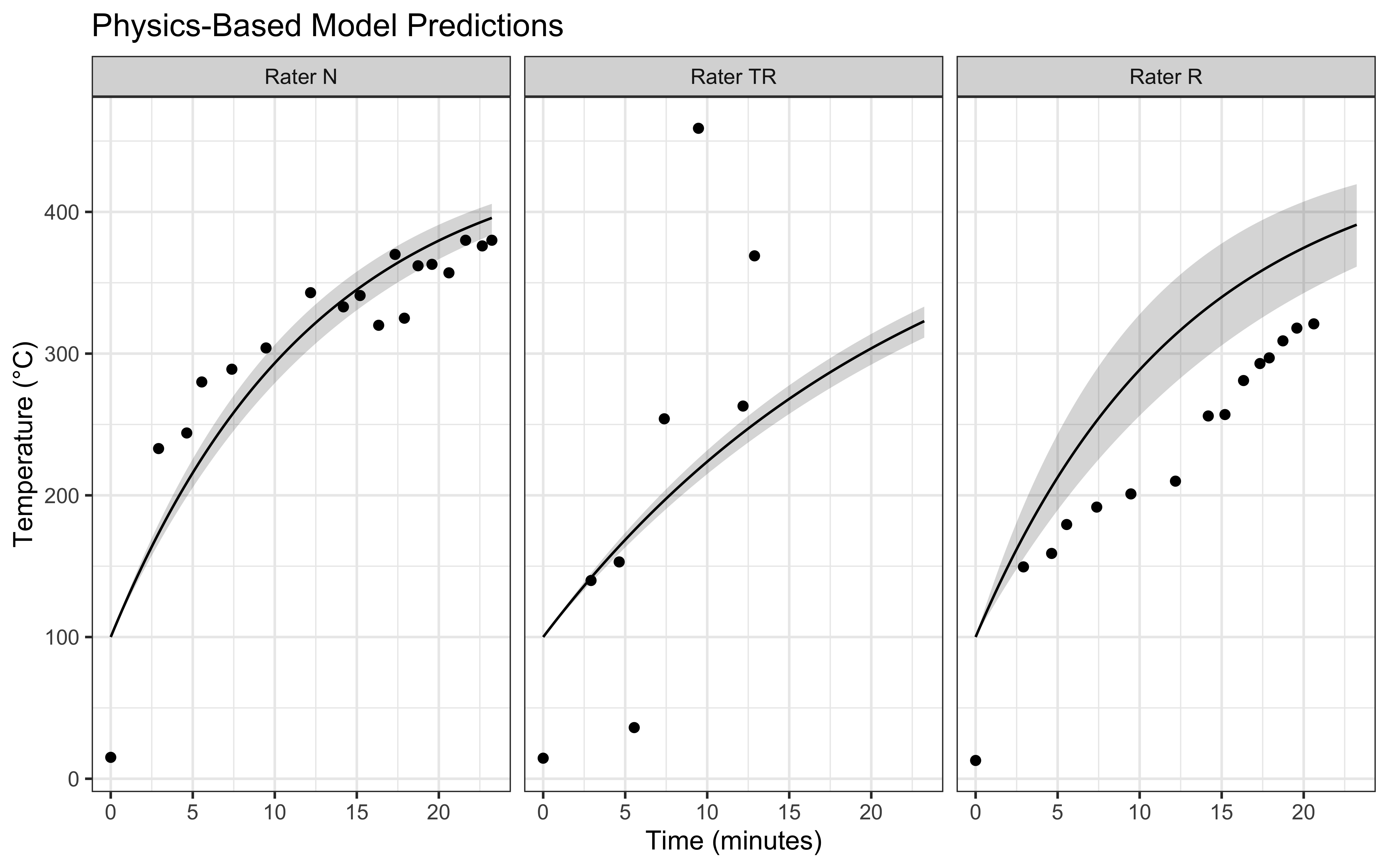
Our implementation combines the theoretical understanding developed in Part 3 with practical considerations for real-world data analysis. The model accounts for measurement uncertainty while maintaining the fundamental physics of heat transfer, providing a robust framework for understanding pizza stone temperature evolution.
2.8 Part 5: Model Analysis and Practical Applications
Having fitted our physics-based model, we must first verify that it actually describes the data well (Validation) before we can use it to make predictions. Once we trust our estimates of the HOT parameter, we can develop practical insights for pizza stone management. A key question for any pizzaiolo is: How long must I wait before the stone is ready? To answer this, we don’t need a new model; we simply need to look at our physics equation from a different angle. By rearranging our original cooling law to solve for time (\(t\)) instead of temperature (\(T\)), we create a predictive tool:
\[t = -\frac{1}{HOT} \ln\left( \frac{T_{\text{target}} - T_{\infty}}{T_{\text{initial}} - T_{\infty}} \right)\]
We will now implement this function in R to calculate precise waiting times under different conditions.
time_to_temp <- function(target_temp, HOT, Ti, Tinf) {
  # Solve: target = Tinf + (Ti - Tinf) * exp(-HOT * t)
  # for t
  t = -1/HOT * log((target_temp - Tinf)/(Ti - Tinf))
  return(t/60)  # Convert seconds to minutes
}
To understand heating times across different oven conditions, we examine how varying flame temperatures affect the time needed to reach pizza-making temperatures. We extract the heating coefficients from our fitted model and analyze temperature scenarios:
# Extract HOT samples from our posterior
hot_samples <- as_draws_df(fit$draws()) %>%
  dplyr::select(starts_with("HOT"))

# Create prediction grid for different flame temperatures
pred_data <- tidyr::crossing(
  Tinf = seq(450, 1200, by = 50),  # Range of flame temperatures
  rater = 1:3
) %>%
  mutate(
    Ti = stan_data$Ti[rater],
    target_temp = 400  # Target temperature for pizza cooking
  )

# Calculate heating times across conditions
n_samples <- 100
time_preds <- map_dfr(1:nrow(pred_data), function(i) {
  times <- sapply(1:n_samples, function(j) {
    hot <- hot_samples[j, paste0("HOT[", pred_data$rater[i], "]")][[1]]
    time_to_temp(
      pred_data$target_temp[i],
      hot,
      pred_data$Ti[i],
      pred_data$Tinf[i]
    )
  })

  data.frame(
    rater = pred_data$rater[i],
    Tinf = pred_data$Tinf[i],
    mean_time = mean(times),
    lower = quantile(times, 0.025),
    upper = quantile(times, 0.975)
  )
})

# Visualize heating time predictions
ggplot(time_preds, aes(x = Tinf)) +
  geom_ribbon(aes(ymin = lower, ymax = upper), alpha = 0.2) +
  geom_line(aes(y = mean_time)) +
  facet_wrap(~rater, labeller = labeller(rater = c(
    "1" = "Rater N",
    "2" = "Rater TR",
    "3" = "Rater R"
  ))) +
  labs(
    title = "Time Required to Reach Pizza-Making Temperature",
    subtitle = "Target temperature: 400°C",
    x = "Flame Temperature (°C)",
    y = "Minutes to reach target"
  ) +
  theme_bw()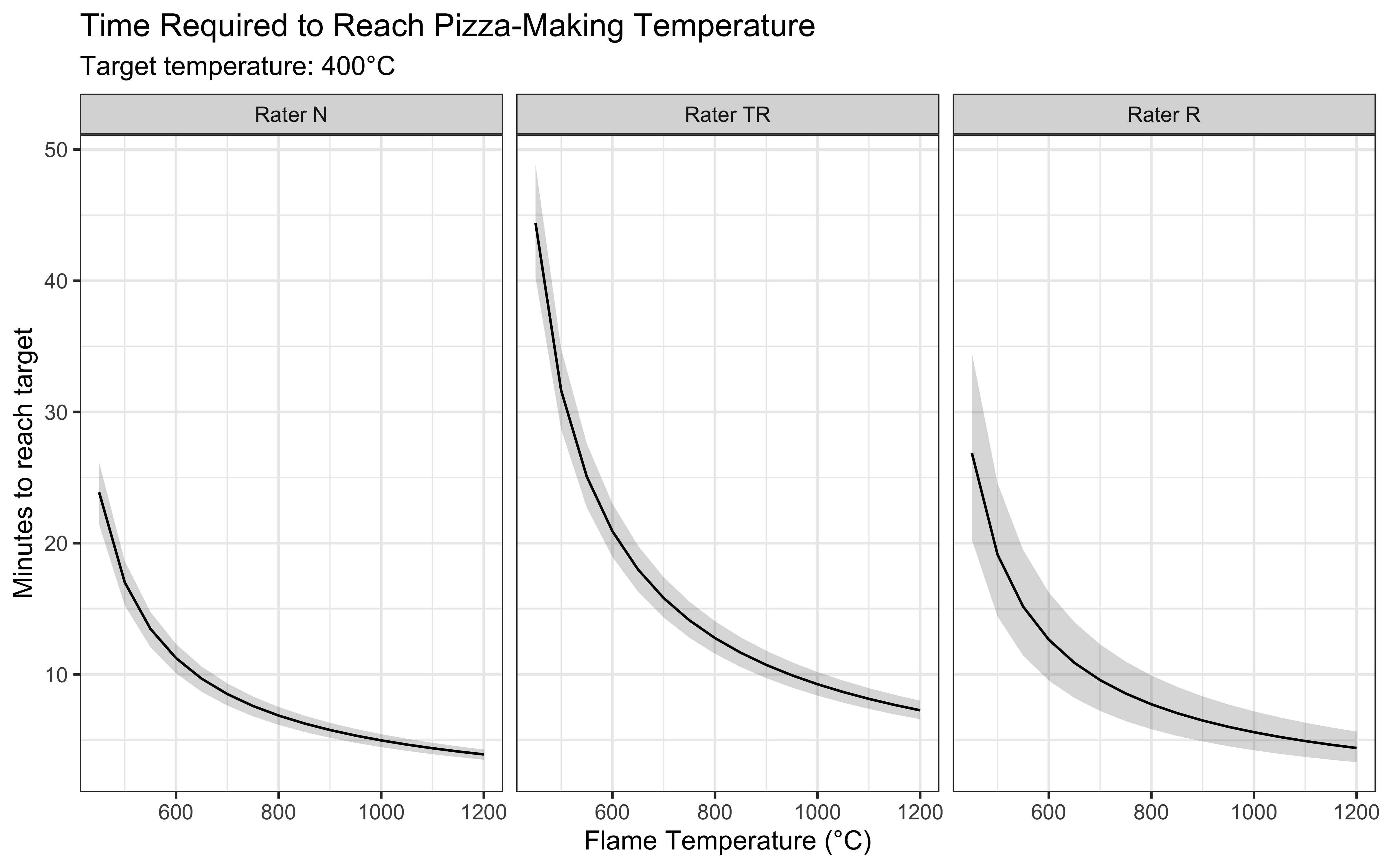
Our analysis reveals several important insights for practical pizza making. First, the heating time decreases non-linearly with flame temperature, showing diminishing returns at very high temperatures. We also observed differences between raters in their measured heating times. These variations likely stem from differences in measurement technique and location on the stone, highlighting the importance of consistent temperature monitoring practices. E.g. N measure the temperature at the boundary between flame and stone, which matches the model’s assumptions better than R, who measures at the center of the stone.
For practical application, we can provide specific heating guidelines based on our model. At a typical flame temperature of 800°C, the model predicts it will take approximately 20-30 minutes to reach optimal pizza-making temperature, assuming room temperature start. However, this time can vary significantly based on:
- Initial stone temperature
- Flame temperature and consistency
- Environmental conditions.
However, we should also consider that the model best fits the measurements from Rater N, who measured at the boundary between flame and stone. This suggests that our predictions are most applicable to the border of the stone, and less to the center (measured by R). Yet, it is the center of the stone that is a better index of the temperature all of our pizza will receive. Therefore we should add a few minutes to the model estimates to ensure best real-world outcomes.
Can we really wait that long? Well, there are no shortcuts to the perfect crust! Just like there is no shortcut to understanding human cognition, and models need always to be critically contextualized in the real world.
2.9 Conclusion: From Pizza to Cognitive Principles
The journey from modeling a heating pizza stone to understanding cognitive processes might seem unusual, but it illustrates fundamental principles that will guide us throughout this course.
Through this seemingly simple physics problem, we have encountered core challenges faced daily by cognitive modelers:
Levels of Analysis: We saw how simplifying complex equations (heat diffusion) mirrors the need to choose the right level of abstraction when modeling cognition (e.g., neural vs. behavioral).
Prior Knowledge: We used physics laws to build a generative model, much like cognitive theories guide model development.
Validation: We confronted the necessity of comparing model predictions to real data, a process central to testing theories.
Parameter Estimation: We used the model to quantify an unobservable property (HOT) from noisy data, analogous to estimating latent cognitive parameters like learning rates or decision thresholds.
Crucially, the comparison between purely statistical models (linear/lognormal) and the physics-based Stan model highlighted the value of mechanistic understanding. While the statistical models struggled to capture the saturation curve — often predicting impossible temperatures via extrapolation — the physics model offered deeper insight and robust predictions. This is a primary goal in cognitive modeling: we do not simply to describe which decisions were made, but we want to capture the underlying mechanism that can increase our understanding of how decisions were made, and generalize to novel unseen decisions.
The pizza stone experiment also demonstrated the importance of rigorous methodology. We saw how multiple measurements from different raters revealed variability in our data, leading us to consider models assumptions, measurement error and individual differences—themes that will become crucial when studying human behavior.
2.10 The Course Roadmap
As we progress through the course, the principles from this chapter will resurface at every step: a generative model driven by theory (Ch. 3), parameter estimation via Bayesian inference (Ch. 4), validation of that inference (Ch. 5), and scaling to many participants (Ch. 6). The pizza stone is not a detour — it is the template.
Every chapter is one step in a single pipeline [NOW COVERING UP TO MODEL COMPARISON. MORE TO COME]. Use this table to orient yourself whenever you feel lost.
| Chapter | Step | Central question |
|---|---|---|
| 1 — Pizza Experiment | Why model? | What is a generative model and what does it mean to fit one to data? |
| 2 — Building Models | Observe & theorize | What behaviors do we see, and what verbal strategies could explain them? |
| 3 — Formal Models | Formalize & simulate | Can we turn a verbal strategy into code that generates realistic data? |
| 4 — Inferring Rates | Fit a single dataset | Given observed data, can we infer the parameters that produced it? |
| 5 — Model Quality | Validate the engine | Are our parameter estimates actually trustworthy? (Prior checks, recovery, SBC, posterior checks) |
| 6 — Multilevel Models | Scale to populations | How do individuals differ, and how do we pool information across them? |
| 7 — Model Comparison | Choose between theories | Of several plausible models, which one best predicts unseen data? |
The key insight: steps 1–3 build models; steps 4–7 test them. A model only earns the right to touch real human data after passing the validation battery in Chapter 5.
Coming up in Chapter 2: We shift focus from stones to minds. You have already played the Matching Pennies game in class. Chapter 2 helps you translate what you observed — your own strategies, your opponent’s patterns — into candidate verbal models that Chapter 3 will then formalize in code.
I hope this has whetted your appetite – both for pizza and for computational modeling!