Chapter 13 Prototype-Based Models of Categorization
13.1 Rethinking Category Representation: From Examples to Averages
In the previous chapter, we explored the Generalized Context Model (GCM), an exemplar model where every encountered example is stored in memory. This approach is powerful but raises questions about cognitive efficiency. Do we really store every single instance we encounter? Consider learning about common categories like “birds” or “chairs”. While specific examples matter, we also seem to develop a general sense of what constitutes a typical member. Prototype theory offers an alternative perspective: instead of storing individual exemplars, the mind abstracts a summary representation — a prototype — for each category. This prototype often represents the central tendency or “average” member.
13.2 Core Ideas of Prototype Models:
Abstraction, Not Storage: The primary representation is a summary (the prototype), not a collection of instances.
Cognitive Economy: Storing one prototype per category is potentially much more memory-efficient than storing numerous exemplars.
Similarity to Prototype: New items are categorized based on their similarity to the stored prototypes of different categories.
Typicality: Items closer to a category’s prototype are judged as more “typical” members and are often categorized faster and more accurately. This contrasts with exemplar models, which emphasize detailed memory for specific instances.
Representation | Abstract summary (e.g., average) | Collection of individual examples |
Memory Cost | Low (one prototype per category) | High (potentially all examples) |
Key Information | Central tendency & variance | Specific instances & their labels |
Sensitivity | Less sensitive to specific examples | Highly sensitive to specific examples |
13.3 Modeling Dynamic Prototypes: The Kalman Filter
Early prototype models often calculated a static average. However, human learning is dynamic; our understanding evolves with experience. How can we model a prototype that updates incrementally as new examples are encountered? The Kalman filter provides a suitable mathematical framework. Originally developed for tracking physical systems amidst noise, it’s well-suited for modeling prototype learning because it allows us to:
Track an Estimate: The category prototype (its average feature values).
Represent Uncertainty: Maintain not just the prototype’s location but also our uncertainty about it.
Update Incrementally: Refine the prototype with each new example.
Balance Old and New: Optimally combine the current prototype (prior belief) with the new example (evidence).
Implement an Adaptive Learning Rate: Automatically adjust how much influence a new example has (the “Kalman gain”) based on current uncertainty. Learning is faster when uncertainty is high and slows as confidence grows.
13.3.1 The Kalman Filter Logic: Updating an Estimate
Imagine tracking a prototype based on a single feature (e.g., average height). The Kalman filter maintains:
Estimate (\(\mu\)): The current best guess for the prototype’s feature value.
Uncertainty (\(\sigma^2\)): The variance around that estimate (higher variance = more uncertainty).
When a new category member (observation x) arrives, we update \(\mu\) and \(\sigma^2\):
- Calculate Kalman Gain (K): This determines the learning rate, balancing current uncertainty (\(\sigma^2_{prev}\)) and assumed observation noise (\(R\), variance of observations around the true prototype): \(K = \frac{\sigma^2_{prev}}{\sigma^2_{prev} + R}\)
** If uncertainty (\(\sigma^2_{prev}\)) is high, \(K\) is large \(\implies\) trust the new observation more.
** If uncertainty is low, \(K\) is small \(\implies\) stick closer to the current estimate.
- Update Estimate (\(\mu\)): Move the old estimate towards the new observation, weighted by the gain: \(\mu_{new} = \mu_{prev} + K \cdot (x - \mu_{prev})\)
** The term \((x - \mu_{prev})\) is the “prediction error” or “innovation”.
- Update Uncertainty (\(\sigma^2\)): Uncertainty always decreases (or stays the same) after incorporating an observation: \(\sigma^2_{new} = (1 - K) \cdot \sigma^2_{prev}\)
This process repeats for every new example belonging to that category.
13.3.2 Extending to Multiple Features: Multivariate Kalman Filter
Our stimuli have two features (height and position). We need a multivariate version:
Estimate (\(\vec{\mu}\)): Now a vector of means (e.g., \([\mu_{height}, \mu_{position}]\)).
Uncertainty (\(\Sigma\)): Now a covariance matrix, capturing variance in each dimension and the covariance between dimensions.
Observation Noise (\(R\)): Also a covariance matrix, representing noise in observing features. Often simplified to a diagonal matrix, assuming independent noise per feature.
Kalman Gain (\(K\)): Now a matrix.
The update equations become matrix operations:
Kalman Gain (\(K\)): \(K = \Sigma_{prev} (\Sigma_{prev} + R)^{-1}\)
Update Estimate (\(\vec{\mu}\)): \(\vec{\mu}{new} = \vec{\mu}{prev} + K (\vec{x} - \vec{\mu}_{prev})\)
Update Uncertainty (\(\Sigma\)): (Using the robust “Joseph form”) \(\Sigma_{new} = (I - K) \Sigma_{prev} (I - K)^T + K R K^T\) (Where \(I\) is the identity matrix)
13.3.3 Implementing the Multivariate Update in R
Let’s write an R function for this multivariate update step.
# Function for one update step of a multivariate Kalman filter
multivariate_kalman_update <- function(mu_prev, # Vector of previous means
                                       sigma_prev, # Previous covariance matrix
                                       observation, # Vector of observed features
                                       r_matrix # Observation noise matrix
                                       ) {
  # Ensure inputs are numeric/matrix
  mu_prev <- as.numeric(mu_prev)
  observation <- as.numeric(observation)
  sigma_prev <- as.matrix(sigma_prev)
  r_matrix <- as.matrix(r_matrix)

  n_dim <- length(mu_prev)
  I <- diag(n_dim) # Identity matrix

  # Calculate Kalman gain (K)
  # Use tryCatch for potential numerical issues during inversion
  combined_cov <- sigma_prev + r_matrix
  S_inv <- tryCatch(solve(combined_cov), error = function(e) {
      warning("Matrix inversion failed (possibly singular). Using pseudo-inverse.", call. = FALSE)
      MASS::ginv(combined_cov) # Fallback using pseudo-inverse
  })
  k_matrix <- sigma_prev %*% S_inv

  # Update mean (mu)
  innovation <- observation - mu_prev # Prediction error
  mu_new <- mu_prev + k_matrix %*% innovation

  # Update covariance (sigma) using Joseph form for numerical stability
  IK_term <- (I - k_matrix)
  sigma_new <- IK_term %*% sigma_prev %*% t(IK_term) + k_matrix %*% r_matrix %*% t(k_matrix)

  # Ensure symmetry (numerical precision can sometimes cause minor asymmetry)
  sigma_new <- (sigma_new + t(sigma_new)) / 2

  return(list(mu = as.numeric(mu_new), sigma = sigma_new, k = k_matrix))
}
This function performs a single update for one category’s prototype when it observes a new member.
13.4 Building the Full Categorization Model
Now we integrate this update mechanism into a full agent that learns prototypes for two categories and makes categorization decisions.
13.4.1 Initialization
We need separate prototypes (\(\mu_0, \Sigma_0\) and \(\mu_1, \Sigma_1\)) for Category 0 and Category 1.
We start with high uncertainty (large initial \(\Sigma\)) and potentially uninformative means (e.g., center of the feature space or rep(0, n_features)).
We need to define the observation noise matrix \(R\). For simplicity, we’ll assume independent noise with the same variance \(r_{val}\) for each feature: \(R = \text{diag}(r_{val}, r_{val})\). The parameter \(r_{val}\) represents how much variability we assume exists within categories or in our perception of the stimuli.
13.4.2 Categorization Decision
How does the model decide the category for a new stimulus \(\vec{x}\)? It compares \(\vec{x}\) to both prototypes, considering their current means (\(\vec{\mu}\)) and uncertainties (\(\Sigma\)). A natural way is to use the probability density of the multivariate normal distribution:
\[P(\vec{x} | \text{Category } C) \propto \exp\left(-\frac{1}{2}(\vec{x} - \vec{\mu}_C)^T (\Sigma_C + R)^{-1} (\vec{x} - \vec{\mu}_C)\right)\]
This essentially calculates how likely the observation \(\vec{x}\) is, given the prototype distribution for category \(C\) (including observation noise \(R\)).
The probability of choosing Category 1 is then calculated using the Luce choice rule (softmax):
\[P(\text{Choose Cat 1} | \vec{x}) = \frac{P(\vec{x} | \text{Category } 1)}{P(\vec{x} | \text{Category } 0) + P(\vec{x} | \text{Category } 1)}\]
We often work with log-probabilities for numerical stability.
13.4.3 The Learning Loop
The agent processes trials sequentially:
Observe stimulus \(\vec{x}_i\).
Calculate \(P(\text{Choose Cat 1} | \vec{x}_i)\) based on current \(\mu_0, \Sigma_0, \mu_1, \Sigma_1\).
Generate a response (e.g., sample from Bernoulli distribution with this probability).
Receive feedback (true category \(y_i\)).
Update the prototype (\(\mu, \Sigma\)) of the correct category \(y_i\) using the multivariate_kalman_update function and \(\vec{x}_i\).
13.4.4 R Implementation of the Prototype Agent
# Prototype model agent using Kalman filter for categorization
prototype_kalman <- function(r_value, # Observation noise variance (scalar)
                             obs, # Matrix of observations (trials x features)
                             cat_one, # Vector of true category labels (0 or 1)
                             initial_mu = NULL, # Optional initial means
                             initial_sigma_diag = 10.0, # Initial uncertainty (diagonal of Sigma)
                             quiet = TRUE) {

  n_trials <- nrow(obs)
  n_features <- ncol(obs)

  # --- Initialization ---
  # Use provided initial means or default to zeros
  if (is.null(initial_mu)) {
    mu0_init <- rep(0, n_features)
    mu1_init <- rep(0, n_features)
  } else {
    # Ensure initial_mu is a list with elements for cat 0 and 1
    mu0_init <- initial_mu[[1]]
    mu1_init <- initial_mu[[2]]
  }

  prototype_cat_0 <- list(
    mu = mu0_init,
    sigma = diag(initial_sigma_diag, n_features)
  )
  prototype_cat_1 <- list(
    mu = mu1_init,
    sigma = diag(initial_sigma_diag, n_features)
  )

  # Observation noise matrix (diagonal)
  r_matrix <- diag(r_value, n_features)

  # Storage for response probabilities
  response_probs <- numeric(n_trials)

  # Log-Sum-Exp function for stable normalization
  log_sum_exp <- function(v) {
    max_v <- max(v)
    max_v + log(sum(exp(v - max_v)))
  }

  # --- Trial Loop ---
  for (i in 1:n_trials) {
    if (!quiet && i %% 10 == 0) print(paste("Trial", i))

    current_obs <- as.numeric(obs[i, ])

    # --- Categorization Decision ---
    # Calculate log probability density for each category prototype

    # Covariance matrix for density calculation (Sigma + R)
    cov_cat_0 <- prototype_cat_0$sigma + r_matrix
    cov_cat_1 <- prototype_cat_1$sigma + r_matrix

    # Use dmvnorm for robust calculation (handles potential issues)
    # Note: We need log probability, so log = TRUE
    log_prob_0 <- tryCatch(
      mvtnorm::dmvnorm(current_obs, mean = prototype_cat_0$mu, sigma = cov_cat_0, log = TRUE),
      error = function(e) -Inf # Return -Inf log prob if density calculation fails
    )
    log_prob_1 <- tryCatch(
      mvtnorm::dmvnorm(current_obs, mean = prototype_cat_1$mu, sigma = cov_cat_1, log = TRUE),
      error = function(e) -Inf
    )

    # Normalize using log-sum-exp to get probability of category 1
    # Handle cases where one log_prob might be -Inf
    if (!is.finite(log_prob_0) && !is.finite(log_prob_1)) {
        prob_cat_1 <- 0.5 # Undefined, default to 0.5
    } else if (!is.finite(log_prob_0)) {
        prob_cat_1 <- 1.0 # Only category 1 has finite probability
    } else if (!is.finite(log_prob_1)) {
        prob_cat_1 <- 0.0 # Only category 0 has finite probability
    } else {
        # Apply bias (b=0.5 means no bias) towards category 1
        b = 0.5
        log_p0_biased = log_prob_0 + log(1-b)
        log_p1_biased = log_prob_1 + log(b)
        prob_cat_1 <- exp(log_p1_biased - log_sum_exp(c(log_p0_biased, log_p1_biased)))
    }

    # Ensure probability is within bounds for rbinom
    response_probs[i] <- max(min(prob_cat_1, 0.9999), 0.0001)

    # --- Learning Update ---
    # Update the prototype for the *correct* category based on feedback
    true_cat <- cat_one[i]

    if (true_cat == 1) {
      update <- multivariate_kalman_update(
        prototype_cat_1$mu,
        prototype_cat_1$sigma,
        current_obs,
        r_matrix
      )
      prototype_cat_1$mu <- update$mu
      prototype_cat_1$sigma <- update$sigma
    } else { # true_cat == 0
      update <- multivariate_kalman_update(
        prototype_cat_0$mu,
        prototype_cat_0$sigma,
        current_obs,
        r_matrix
      )
      prototype_cat_0$mu <- update$mu
      prototype_cat_0$sigma <- update$sigma
    }
  } # End trial loop

  # Return simulated binary responses based on calculated probabilities
  return(rbinom(n_trials, 1, response_probs))
}
13.4.5 Simulating Categorization Behavior
Let’s simulate behavior using this model on the same experimental setup from Chapter 11. The key parameter here is r_value, the observation noise. This parameter reflects the model’s assumption about how much variability exists within categories or arises from perceptual noise.
Low r_value: Model assumes observations are precise representations of the category; prototypes may change rapidly initially but might overfit to early examples.
High r_value: Model assumes observations are noisy; learning is slower as each example has less influence, but the model might generalize better.
# Function to wrap simulation for different parameters
simulate_prototype_responses <- function(agent, r_value, experiment_data) {

    observations <- as.matrix(experiment_data %>% dplyr::select(height, position))
    category <- experiment_data$category

    # Simulate responses using the prototype_kalman function
    responses <- prototype_kalman(
        r_value = r_value,
        obs = observations,
        cat_one = category,
        initial_mu = list(rep(0,2), rep(0,2)), # Start prototypes at 0
        initial_sigma_diag = 10.0, # High initial uncertainty
        quiet = TRUE
    )

    # Record results
    tmp_simulated_responses <- experiment_data %>%
        mutate(
            trial = 1:n(),
            sim_response = responses,
            correct = ifelse(category == sim_response, 1, 0),
            performance = cumsum(correct) / trial,
            r_value = r_value,
            agent = agent
        )

    return(tmp_simulated_responses)
}

# Define parameters for simulation
param_df <- dplyr::tibble(
    expand_grid(
        agent = 1:10, # Simulate 10 agents per condition
        r_value = c(0.1, 0.5, 1.0, 2.0, 5.0) # Different levels of observation noise
    )
)

# Run simulations in parallel
# (Load pre-computed results if regenerate_simulations is FALSE)
sim_file <- "simdata/W12_prototype_simulated_responses.csv"
if (regenerate_simulations || !file.exists(sim_file)) {
  cat("Regenerating prototype simulations...\n")
  plan(multisession, workers = availableCores()) # Ensure parallel plan is active

  # Pass 'experiment' tibble explicitly to the mapping function
  prototype_responses <- future_pmap_dfr(param_df,
      simulate_prototype_responses,
      experiment_data = experiment, # Pass the experiment data here
      .options = furrr_options(seed = TRUE)
  )

  # Create simdata directory if it doesn't exist
  if (!dir.exists("simdata")) dir.create("simdata")
  # Save results
  write_csv(prototype_responses, sim_file)
  cat("Simulations saved.\n")

} else {
  cat("Loading existing prototype simulations...\n")
  prototype_responses <- read_csv(sim_file)
  cat("Simulations loaded.\n")
}
## Loading existing prototype simulations...## Simulations loaded.# Visualize how observation noise affects learning
ggplot(prototype_responses, aes(x = trial, y = performance, color = factor(r_value))) +
stat_summary(fun = mean, geom = "line", alpha = 0.8, linewidth = 1) +
stat_summary(fun.data = mean_se, geom = "ribbon", alpha = 0.15, aes(fill = factor(r_value))) +
theme_bw() +
labs(
title = "Prototype Model Learning Performance",
subtitle = "Effect of Observation Noise (r_value)",
x = "Trial Number",
y = "Proportion Correct (Mean +/- SE)",
color = "r_value",
fill = "r_value"
) +
ylim(0.4, 1.0) # Adjust ylim for better visibility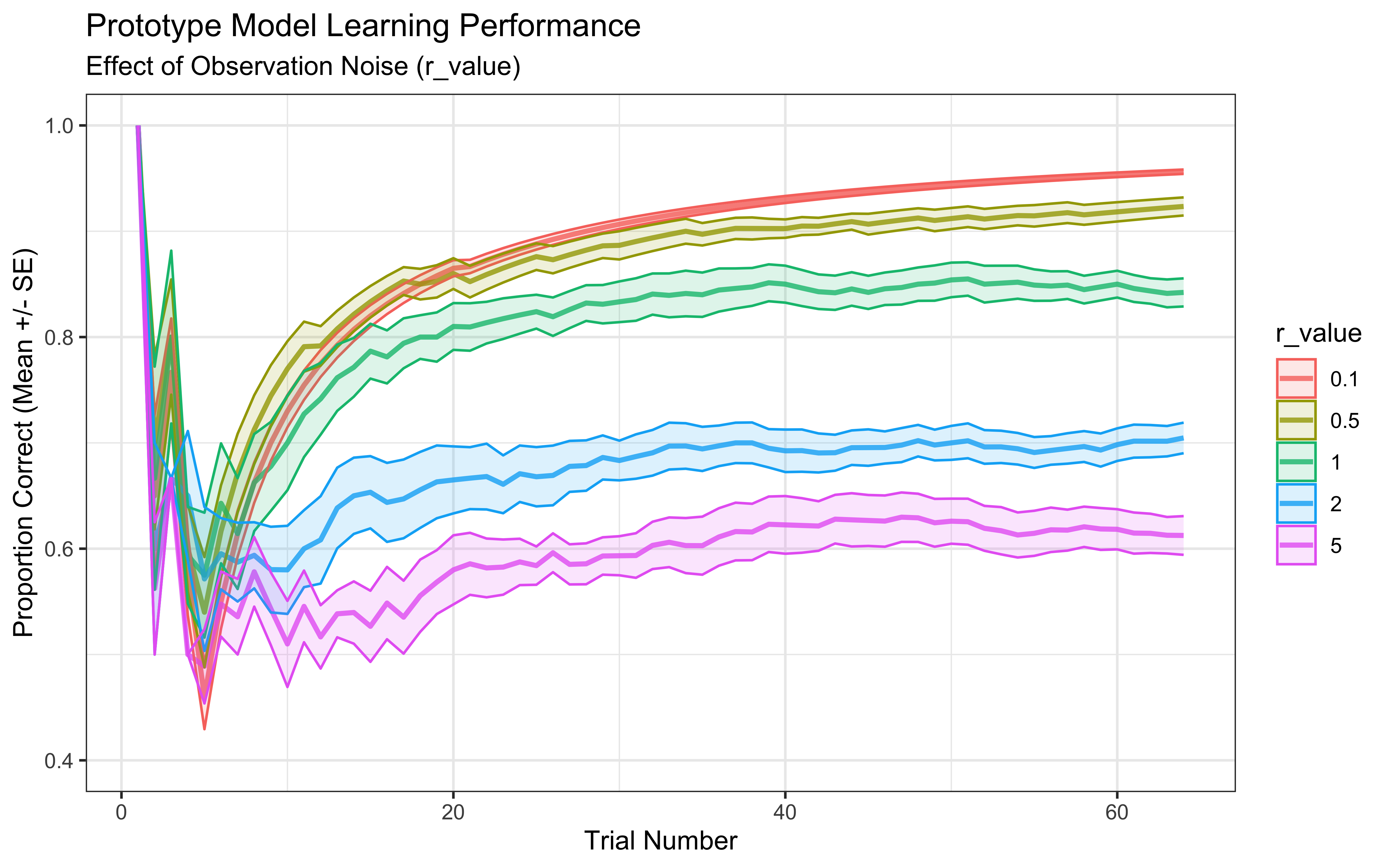
Interpretation: This plot shows average learning curves. Different values of r_value impact learning. Very low noise (r_value = 0.1) might lead to overfitting initial examples, while very high noise (r_value = 5.0) might slow down learning as the model trusts observations less. An intermediate value often performs best, balancing trust in new data with reliance on the established prototype.
13.4.6 Visualizing Prototype Evolution
Where do the prototypes end up? Let’s track their movement and uncertainty over trials.
# Function to track prototype means and covariances over trials
track_prototypes <- function(r_value, obs, cat_one, initial_mu = NULL, initial_sigma_diag = 10.0) {
  n_trials <- nrow(obs)
  n_features <- ncol(obs)

  # --- Initialization ---
  if (is.null(initial_mu)) {
    mu0_init <- rep(2.5, n_features)
    mu1_init <- rep(2.5, n_features)
  } else {
    mu0_init <- initial_mu[[1]]
    mu1_init <- initial_mu[[2]]
  }
  prototype_cat_0 <- list(mu = mu0_init, sigma = diag(initial_sigma_diag, n_features))
  prototype_cat_1 <- list(mu = mu1_init, sigma = diag(initial_sigma_diag, n_features))
  r_matrix <- diag(r_value, n_features)

  # Storage for history
  # Store the full 2x2 covariance matrix in a list column
  prototype_history <- list()

  # --- Trial Loop ---
  for (i in 1:(n_trials + 1)) { # Loop one extra time to capture final state
    # Store current state *before* update (or final state)
     prototype_history[[length(prototype_history) + 1]] <- tibble(
        trial = i, category = 0,
        feature1_mean = prototype_cat_0$mu[1], # Assuming feature 1 is height
        feature2_mean = prototype_cat_0$mu[2], # Assuming feature 2 is position
        cov_matrix = list(prototype_cat_0$sigma)
     )
     prototype_history[[length(prototype_history) + 1]] <- tibble(
        trial = i, category = 1,
        feature1_mean = prototype_cat_1$mu[1],
        feature2_mean = prototype_cat_1$mu[2],
        cov_matrix = list(prototype_cat_1$sigma)
     )

    # Update only if within actual trials
    if (i <= n_trials) {
      current_obs <- as.numeric(obs[i, ])
      true_cat <- cat_one[i]

      if (true_cat == 1) {
        update <- multivariate_kalman_update(prototype_cat_1$mu, prototype_cat_1$sigma, current_obs, r_matrix)
        prototype_cat_1$mu <- update$mu
        prototype_cat_1$sigma <- update$sigma
      } else {
        update <- multivariate_kalman_update(prototype_cat_0$mu, prototype_cat_0$sigma, current_obs, r_matrix)
        prototype_cat_0$mu <- update$mu
        prototype_cat_0$sigma <- update$sigma
      }
    }
  } # End trial loop

  return(bind_rows(prototype_history)) # Combine list into single tibble
}

# Helper function to get ellipse data for plotting uncertainty
# Requires the 'ellipse' package
get_ellipse <- function(mu, sigma, level = 0.68) { # 68% CI (approx 1 SD)
  if (!requireNamespace("ellipse", quietly = TRUE)) {
    warning("Package 'ellipse' needed for uncertainty ellipses.", call. = FALSE)
    return(NULL)
  }
  mu <- as.numeric(mu)
  sigma <- as.matrix(sigma)
  if (length(mu) != 2 || !all(dim(sigma) == c(2,2))) {
      warning("Ellipse plotting requires 2D mean vector and 2x2 covariance matrix.", call. = FALSE)
      return(NULL)
  }
  # Check positive definiteness for ellipse calculation
  eigen_vals <- eigen(sigma, symmetric = TRUE, only.values = TRUE)$values
  if (any(eigen_vals <= 1e-6)) {
      # warning("Covariance matrix near non-positive definite. Adding jitter for ellipse.", call. = FALSE)
      sigma <- sigma + diag(ncol(sigma)) * 1e-6 # Add tiny jitter
  }

  # Calculate points on the ellipse boundary
  ellipse_points <- tryCatch(ellipse::ellipse(sigma, centre = mu, level = level),
                             error = function(e) {
                                 warning(paste("Ellipse calculation failed:", e$message), call. = FALSE)
                                 NULL
                             })
  if (is.null(ellipse_points)) return(NULL)
  # Return as tibble with consistent names (feature1=height, feature2=position)
  tibble::as_tibble(ellipse_points) %>% setNames(c("feature1_mean", "feature2_mean"))
}


# --- Run tracking and prepare plot data ---
# Track prototypes using the actual experiment data
prototype_trajectory <- track_prototypes(
  r_value = 1.0, # Example r_value
  obs = as.matrix(experiment[, c("height", "position")]),
  cat_one = experiment$category,
  initial_mu = list(rep(2.5,2), rep(2.5,2)), # Start at 0
  initial_sigma_diag = 10.0
)

# Get final prototype states (after the last update, trial = n_trials + 1)
final_prototypes <- prototype_trajectory %>% filter(trial == max(trial))

# Create ellipse data for the final states
# Use rowwise and map to handle list column 'cov_matrix'
ellipse_data_list <- final_prototypes %>%
  rowwise() %>%
  mutate(ellipse_df = list(get_ellipse(c(feature1_mean, feature2_mean), cov_matrix[[1]]))) %>%
  ungroup() %>%
  filter(!sapply(ellipse_df, is.null)) # Remove rows where ellipse failed

# Check if ellipse data was successfully generated
if (nrow(ellipse_data_list) > 0) {
    ellipse_data_unnested <- ellipse_data_list %>%
      dplyr::select(category, ellipse_df) %>% # Select only needed columns
      unnest(ellipse_df)
} else {
    warning("Could not generate ellipse data for plotting.", call. = FALSE)
    ellipse_data_unnested <- NULL # Set to NULL if empty
}


# --- Create the Plot ---
p_trajectory <- ggplot() +
  # Plot stimuli points (make them slightly transparent)
  geom_point(data = stimuli,
             aes(x = position, y = height, color = factor(category), shape = factor(category)),
             size = 3, alpha = 0.5) +

  # Plot prototype trajectory path (use trial <= n_trials for the path itself)
  geom_path(data = prototype_trajectory %>% filter(trial <= nrow(experiment)),
            aes(x = feature2_mean, y = feature1_mean, group = category, color = factor(category)),
            linetype = "dashed",
            arrow = arrow(type = "closed", length = unit(0.08, "inches"), angle = 20)) +

  # Plot final prototype means (points at the end of the path)
  geom_point(data = final_prototypes,
             aes(x = feature2_mean, y = feature1_mean, color = factor(category)),
             size = 4, shape = 18) # Use a different shape for final point

# Add ellipses if data exists
if (!is.null(ellipse_data_unnested)) {
  # Plot ellipses using geom_path, mapping x to feature2_mean and y to feature1_mean
  p_trajectory <- p_trajectory +
    geom_path(data = ellipse_data_unnested,
              aes(x = feature2_mean, y = feature1_mean, group = category, color = factor(category)),
              alpha = 0.7, linewidth = 0.8)
}

# Add labels and theme
p_trajectory <- p_trajectory +
  scale_color_discrete(name = "Category") +
  scale_shape_discrete(name = "Category") +
  labs(
    title = "Prototype Learning Trajectory (Kalman Filter)",
    subtitle = "Prototypes start at (2.5,2.5). Dashed lines show path, ellipses show final 68% uncertainty.",
    x = "Position Feature",
    y = "Height Feature"
  ) +
  theme_bw() +
  # Set coordinate limits to ensure all points/paths are visible
  coord_cartesian(xlim = range(c(stimuli$position, prototype_trajectory$feature2_mean), na.rm = TRUE) + c(-0.5, 0.5),
                  ylim = range(c(stimuli$height, prototype_trajectory$feature1_mean), na.rm = TRUE) + c(-0.5, 0.5))

# Print the final plot
print(p_trajectory)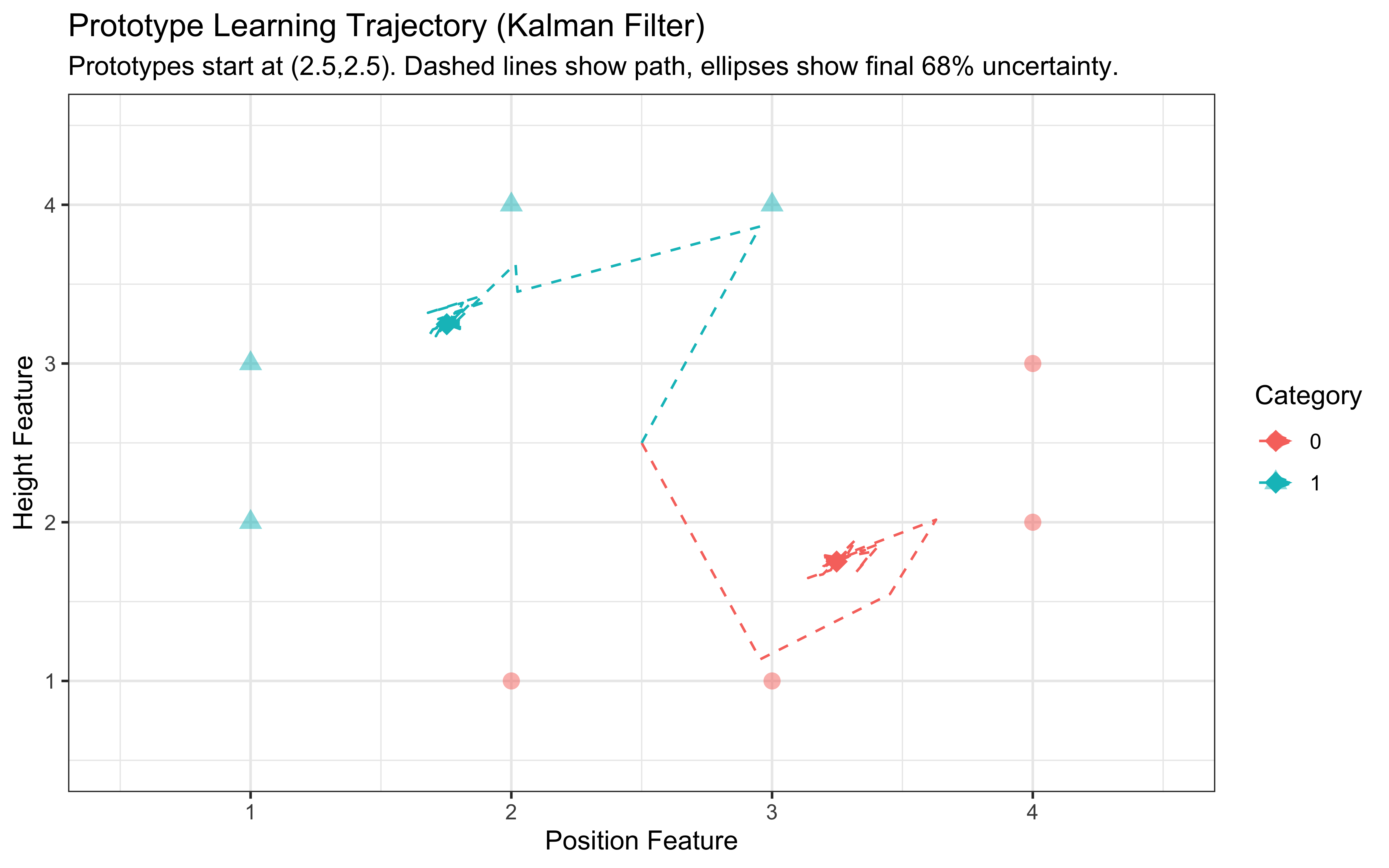
Interpretation: This plot shows the stimuli (circles/triangles) and the path the prototypes took during learning (dashed lines starting in the middle). The final prototype locations are marked with diamonds, and the ellipses represent the model’s final uncertainty (68% confidence interval) about the true prototype location for each category. We see the prototypes moving towards the center of their respective category members and uncertainty shrinking over time (though the ellipses represent only the final uncertainty).
13.5 Estimating Parameters: Implementing the Prototype Model in Stan
Simulations help us understand the model, but we usually want to fit the model to real experimental data to estimate its parameters. Here, the key free parameter is the observation noise variance, r_value. We’ll implement the Kalman filter prototype model in Stan to estimate r_value from data.
13.5.1 The Stan Model (W12_prototype_single.stan)
The Stan code mirrors the logic of our R simulation (prototype_kalman) but within Stan’s framework for Bayesian inference. The Stan code needs to replicate the trial-by-trial Kalman filter process within its transformed parameters block to calculate the choice probabilities, which are then used in the model block to compare against observed choices (y). We estimate r_value (specifically, log_r for better sampling).
prototype_single_stan <- "
// Stan Code for Prototype Model using Kalman Filter (W12_prototype_single.stan)

data {
  int<lower=1> ntrials;                // Number of trials
  int<lower=1> nfeatures;              // Number of feature dimensions (e.g., 2)
  array[ntrials] int<lower=0, upper=1> cat_one;  // True category labels (0 or 1) provided as feedback
  array[ntrials] int<lower=0, upper=1> y;        // Observed participant decisions (0 or 1)
  array[ntrials, nfeatures] real obs;  // Stimulus features (trials x features)

  // Priors / Fixed Values
  real<lower=0, upper=1> b;            // Response bias (e.g., 0.5 for no bias)
  vector[nfeatures] initial_mu_cat0;   // Initial mean vector for prototype 0
  vector[nfeatures] initial_mu_cat1;   // Initial mean vector for prototype 1
  real<lower=0> initial_sigma_diag;    // Initial diagonal value for covariance matrices

  // Prior parameters for log_r
  real prior_logr_mean;
  real<lower=0> prior_logr_sd;
}

parameters {
  // Parameter to estimate: Observation noise variance on log scale
  real log_r;
}

transformed parameters {
  // Transform log_r to observation noise variance (r_value)
  // Using exp() ensures positivity. Add a small epsilon for stability if needed.
  real<lower=1e-6> r_value = exp(log_r);

  // Store response probabilities for each trial
  array[ntrials] real<lower=0.0001, upper=0.9999> p; // Prob of choosing category 1

  // --- Kalman Filter Simulation within Stan ---
  // Initialize prototypes (means and covariance matrices)
  vector[nfeatures] mu_cat0 = initial_mu_cat0;
  vector[nfeatures] mu_cat1 = initial_mu_cat1;
  matrix[nfeatures, nfeatures] sigma_cat0 = diag_matrix(rep_vector(initial_sigma_diag, nfeatures));
  matrix[nfeatures, nfeatures] sigma_cat1 = diag_matrix(rep_vector(initial_sigma_diag, nfeatures));

  // Observation noise matrix (diagonal)
  matrix[nfeatures, nfeatures] r_matrix = diag_matrix(rep_vector(r_value, nfeatures));
  matrix[nfeatures, nfeatures] I = diag_matrix(rep_vector(1.0, nfeatures)); // Identity matrix

  // Process trials sequentially
  for (i in 1:ntrials) {
    vector[nfeatures] current_obs = to_vector(obs[i]);

    // --- Categorization Decision Probability ---
    matrix[nfeatures, nfeatures] cov_cat0 = sigma_cat0 + r_matrix;
    matrix[nfeatures, nfeatures] cov_cat1 = sigma_cat1 + r_matrix;

    // Calculate log probability densities using multi_normal_lpdf for robustness
    // Add bias term b (log(b) for cat 1, log(1-b) for cat 0)
    real log_p0 = multi_normal_lpdf(current_obs | mu_cat0, cov_cat0) + log(1 - b);
    real log_p1 = multi_normal_lpdf(current_obs | mu_cat1, cov_cat1) + log(b);

    // Calculate probability of choosing category 1 using log_sum_exp
    real log_sum_p = log_sum_exp(log_p0, log_p1);
    real prob_cat_1 = exp(log_p1 - log_sum_p);

    // Bound probabilities away from 0 and 1 for numerical stability
    p[i] = fmax(fmin(prob_cat_1, 0.9999), 0.0001);

    // --- Learning Update (based on true feedback cat_one[i]) ---
    // Only update if it's not the very last observation
    // (or adjust loop if feedback influences next trial's decision directly)
    // This logic assumes decision P is based on state *before* update for trial i.
    if (i < ntrials) { // Optional: only update if there are future trials
      if (cat_one[i] == 1) { // Update prototype 1
        vector[nfeatures] innovation = current_obs - mu_cat1;
        matrix[nfeatures, nfeatures] S = sigma_cat1 + r_matrix;
        // Use mdivide_right_spd for K = Sigma * S^-1 (more stable)
        matrix[nfeatures, nfeatures] K = mdivide_right_spd(sigma_cat1, S);
        mu_cat1 = mu_cat1 + K * innovation;
        matrix[nfeatures, nfeatures] IK = I - K;
        // Joseph form update for sigma
        sigma_cat1 = IK * sigma_cat1 * IK' + K * r_matrix * K';
      } else { // Update prototype 0
        vector[nfeatures] innovation = current_obs - mu_cat0;
        matrix[nfeatures, nfeatures] S = sigma_cat0 + r_matrix;
        matrix[nfeatures, nfeatures] K = mdivide_right_spd(sigma_cat0, S);
        mu_cat0 = mu_cat0 + K * innovation;
        matrix[nfeatures, nfeatures] IK = I - K;
        sigma_cat0 = IK * sigma_cat0 * IK' + K * r_matrix * K';
      }
       // Ensure symmetry after update (optional but good practice)
       sigma_cat0 = 0.5 * (sigma_cat0 + sigma_cat0');
       sigma_cat1 = 0.5 * (sigma_cat1 + sigma_cat1');
    }
  }
}

model {
  // Prior for the observation noise parameter (on log scale)
  target += normal_lpdf(log_r | prior_logr_mean, prior_logr_sd);

  // Likelihood: Observed decisions y follow a Bernoulli distribution
  // with probabilities p calculated in transformed parameters
  target += bernoulli_lpmf(y | p);
}

generated quantities {
  // Calculate log likelihood for each trial for model comparison (e.g., LOO)
  array[ntrials] real log_lik;
  for (i in 1:ntrials) {
    log_lik[i] = bernoulli_lpmf(y[i] | p[i]);
  }

  // Posterior predictive checks: simulate data based on estimated parameters
  array[ntrials] int y_pred;
  for (i in 1:ntrials) {
    y_pred[i] = bernoulli_rng(p[i]);
  }

  // Save estimated r_value on original scale
  real estimated_r_value = r_value;
}"

# Write the model to a file
write_stan_file(
  prototype_single_stan,
  dir = "stan/",
  basename = "W12_prototype_single.stan"
)
## [1] "/Users/au209589/Dropbox/Teaching/AdvancedCognitiveModeling23_book/stan/W12_prototype_single.stan"# Compile the Stan model using cmdstanr
# This might take a minute or two the first time it's run
mod_prototype_single <- cmdstan_model(
file.path("stan/W12_prototype_single.stan"),
cpp_options = list(stan_threads = TRUE)
)
cat("Stan model compiled successfully.\n")## Stan model compiled successfully.Key aspects of the Stan implementation:
Data: Takes trial-by-trial observations (obs), true categories (cat_one for updates), and participant responses (y). Also requires initial prototype states and prior parameters.
Parameters: Estimates log_r, the logarithm of the observation noise variance. Estimating on the log scale helps with sampling as variance must be positive.
Transformed Parameters:
** Calculates r_value = exp(log_r).
** Re-simulates the Kalman filter trial-by-trial, updating mu and sigma based on cat_one.
** Calculates the probability p[i] of choosing Category 1 for each trial before the update for that trial, using the current mu, sigma, and estimated r_value.
- Model Block:
** Sets a prior on log_r (e.g., normal(0, 1), meaning r_value is centered around exp(0)=1).
** Defines the likelihood using bernoulli_lpmf(y | p), stating that the observed responses y are Bernoulli distributed with the calculated probabilities p.
- Generated Quantities: Calculates log-likelihood for model comparison and generates posterior predictions (y_pred).
13.5.2 Parameter Recovery: Can We Retrieve the Noise Parameter?
A crucial check is parameter recovery. If we simulate data with a known r_value, can our Stan model accurately estimate it back?
We will simulate data using the same experimental structure (experiment) and the prototype_kalman R function used earlier. This ensures we test recovery on data generated precisely by the model logic we’re trying to fit.
# Function to run one simulation and prepare Stan data
run_single_recovery_trial <- function(true_r_value, experiment_data) {

  # Simulate responses using prototype_kalman
  sim_responses <- prototype_kalman(
    r_value = true_r_value,
    obs = as.matrix(experiment_data[, c("height", "position")]),
    cat_one = experiment_data$category,
    initial_mu = list(rep(0,2), rep(0,2)),
    initial_sigma_diag = 10.0,
    quiet = TRUE
  )

  # Prepare data list for Stan
  stan_data <- list(
    ntrials = nrow(experiment_data),
    nfeatures = 2,
    cat_one = experiment_data$category,
    y = sim_responses, # Use simulated responses as 'observed' data
    obs = as.matrix(experiment_data[, c("height", "position")]),
    b = 0.5, # No bias
    initial_mu_cat0 = rep(0, 2),
    initial_mu_cat1 = rep(0, 2),
    initial_sigma_diag = 10.0,
    prior_logr_mean = 0, # Prior centered on r_value=1
    prior_logr_sd = 1.0  # Reasonably broad prior
  )

  return(stan_data)
}

# Define true r_values to test
r_values_to_test <- c(0.1, 0.5, 1.0, 2.0, 3.0, 5.0)

# Data frame to store recovery results
recovery_results_list <- list()

# (Load pre-computed results if regenerate_simulations is FALSE)
recovery_file <- "simdata/W12_prototype_recovery_results.rds"
if (regenerate_simulations || !file.exists(recovery_file)) {
  cat("Regenerating parameter recovery simulations...\n")

  # Loop through each true r_value
  for (r_val in r_values_to_test) {
    cat("  Testing r_value =", r_val, "\n")

    # 1. Generate synthetic data for this r_value
    current_stan_data <- run_single_recovery_trial(r_val, experiment)

    # 2. Fit the Stan model (using pre-compiled model)
    fit <- mod_prototype_single$sample(
      data = current_stan_data,
      seed = 123,
      chains = 2, # Use at least 2 chains
      parallel_chains = 2,
      threads_per_chain = 1, # Adjust based on system cores
      iter_warmup = 500, # Reduced iterations for faster recovery check
      iter_sampling = 1000,
      refresh = 0, # Suppress verbose output
      show_messages = FALSE
    )

    # 3. Extract estimated r_value posterior
    # Use the variable saved in generated quantities
    draws <- fit$draws("estimated_r_value", format = "df")
    estimate_mean <- mean(draws$estimated_r_value)
    ci_lower <- quantile(draws$estimated_r_value, 0.025)
    ci_upper <- quantile(draws$estimated_r_value, 0.975)

    # Store results
    recovery_results_list[[length(recovery_results_list) + 1]] <- tibble(
      true_r_value = r_val,
      estimated_r_mean = estimate_mean,
      est_lower_95 = ci_lower,
      est_upper_95 = ci_upper
    )
  } # End loop over r_values

  recovery_results <- bind_rows(recovery_results_list)
  # Save results
  if (!dir.exists("simdata")) dir.create("simdata")
  saveRDS(recovery_results, recovery_file)
  cat("Parameter recovery simulations saved.\n")

} else {
  cat("Loading existing parameter recovery results...\n")
  recovery_results <- readRDS(recovery_file)
  cat("Results loaded.\n")
}
## Loading existing parameter recovery results...
## Results loaded.# --- Visualize parameter recovery ---
ggplot(recovery_results, aes(x = true_r_value, y = estimated_r_mean)) +
geom_abline(intercept = 0, slope = 1, linetype = "dashed", color = "grey50") +
geom_errorbar(aes(ymin = est_lower_95, ymax = est_upper_95), width = 0.1, alpha = 0.6) +
geom_point(size = 3, color = "dodgerblue") +
labs(
title = "Parameter Recovery for Prototype Model (r_value)",
subtitle = "Points are posterior means, bars are 95% Credible Intervals.\nDashed line is perfect recovery.",
x = "True Observation Noise Variance (r_value)",
y = "Estimated Observation Noise Variance"
) +
theme_minimal() +
# Adjust scale if needed, e.g., scale_x_log10() + scale_y_log10() if range is large
coord_cartesian(xlim = range(recovery_results$true_r_value) + c(-0.5, 0.5),
ylim = range(c(recovery_results$est_lower_95, recovery_results$est_upper_95)) + c(-0.5, 0.5) )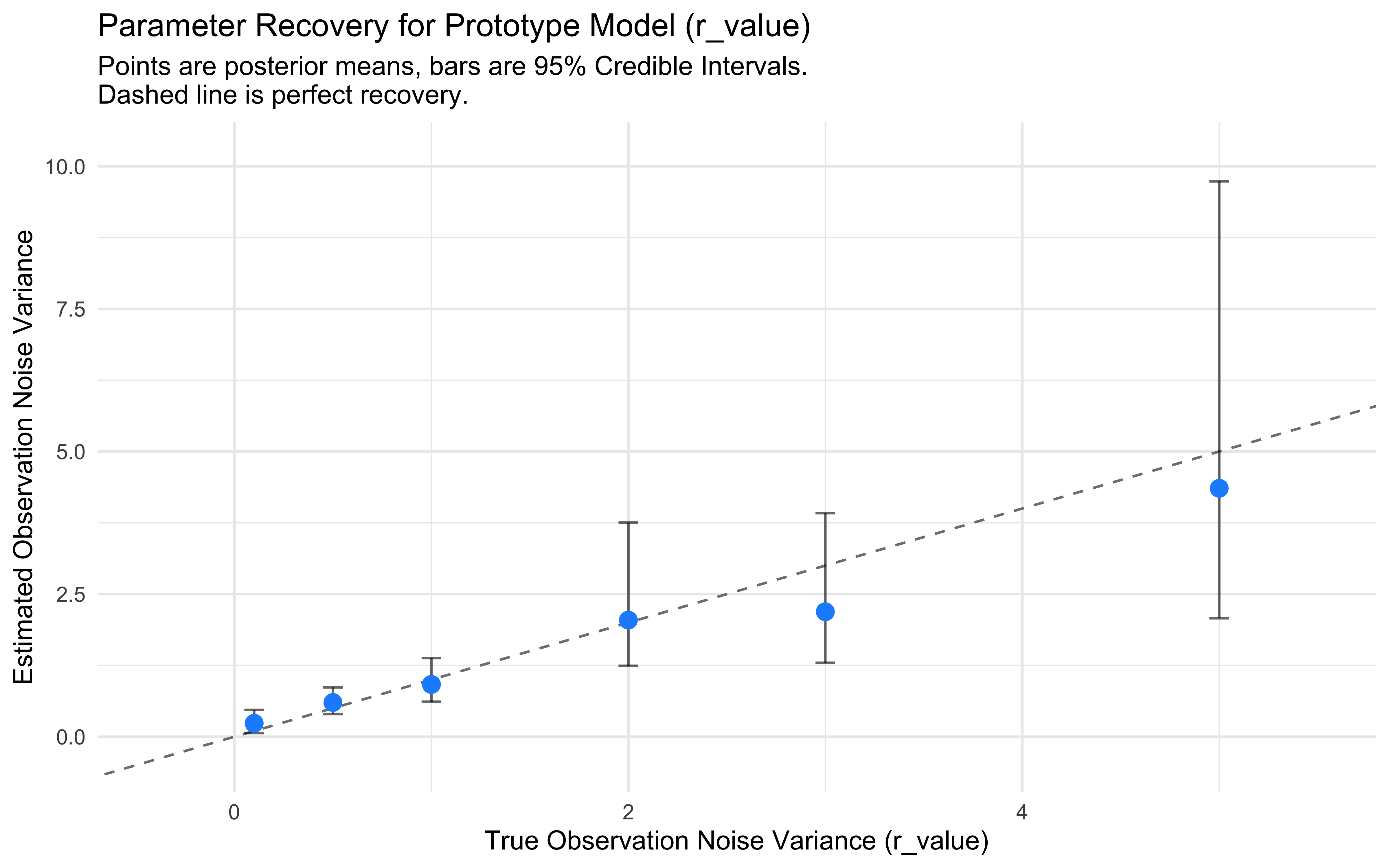
Discussion of Recovery Results: Examine the plot. Ideally, the points should fall close to the dashed diagonal line, and the error bars (95% credible intervals) should overlap the true value.
13.6 Cognitive Insights and Model Comparison
The Kalman filter prototype model offers valuable insights:
Incremental, Adaptive Learning: It formalizes how category knowledge can be built up one example at a time, with learning automatically slowing down as confidence increases. Uncertainty Representation: It explicitly models the learner’s uncertainty about category prototypes.
Memory Efficiency: It achieves learning by storing only summary statistics (mean and covariance) per category, aligning with intuitions about cognitive limits.
13.6.1 Comparing to Exemplar Models (GCM):
The GCM stores every detail; the prototype model abstracts.
The GCM is sensitive to specific outliers; the prototype model is less so (outliers get averaged in).
The GCM requires explicit attention weights; attention in the Kalman filter can emerge implicitly if uncertainty differs across dimensions (though not explored in detail here).
13.6.2 Limitations:
Abstraction Loses Detail: Information about specific examples and category variance beyond the covariance matrix is lost. There are models that try to combine both approaches [MISSING REFS].
Single Prototype: Assumes categories have a single central tendency, struggling with disjunctive categories (e.g., “mammals that fly or swim”). Extensions like multiple-prototype models address this[MISSING REFS].
Conclusion
The Kalman filter prototype model provides a dynamic, computationally plausible account of how categories might be learned by abstracting central tendencies and tracking uncertainty. While parameter estimation can be challenging, the model captures key aspects of incremental learning and memory efficiency. It stands as a compelling alternative to exemplar-based approaches, highlighting the fundamental trade-off between detailed instance memory and abstract summary representation in categorization. The next chapter will introduce a third perspective: rule-based models.