# From simulation to model fitting {#sec-inferring-rates}
```{r ch05_setup, include=FALSE}
knitr::opts_chunk$set(
warning = FALSE,
message = FALSE,
echo = TRUE,
fig.width = 8,
fig.height = 5,
fig.align = 'center',
out.width = "80%",
dpi = 300
)
pacman::p_load(
tidyverse,
here,
cmdstanr,
posterior,
bayesplot,
furrr,
future,
patchwork
)
# Parallel Setup: Leave 2 cores free for system stability
n_cores <- parallel::detectCores() - 2
future::plan(multisession, workers = n_cores)
theme_set(theme_classic())
```
> **📍 Where we are in the Bayesian modeling workflow:**
> Ch. 3 built forward models — code that generates data *from* known parameters.
> This chapter reverses the arrow: given observed choices, we infer the parameters
> that most plausibly produced them. This is **Bayesian parameter estimation**, and
> it is the engine at the heart of all remaining chapters. We fit to *simulated*
> data here precisely because we know the ground truth — a sanity check before the
> engine is handed real human data in Ch. 6.
In Chapter 3, we formalized verbal models into computational agents and explored their behavior through simulation by *setting* their parameters (like bias `rate` or WSLS rules). However, when analyzing real experimental data, we don't know the true parameter values underlying a participant's behavior. The core task shifts from simulation to **parameter estimation**: inferring the plausible values of model parameters *given* the observed data.
## Learning Objectives
This chapter transitions from simulating predefined models (Chapter 3) to inferring model parameters from data using Bayesian methods. By the end of this chapter, you will be able to:
* **Model Cognitive Processes:** Apply these techniques to estimate parameters for simple cognitive strategies, including biased choice and different types of memory models.
* **Master Reparameterization:** Learn to rethink the mathematical form of models. You will appreciate the utility of the log-odds transformation for mapping bounded probability parameters into unbounded spaces.
* **Read MCMC Diagnostics:** Learn the mandatory diagnostic battery for Bayesian inference, specifically focusing on chain convergence ($\hat{R}$) and Effective Sample Size (ESS).
In a rigorous Bayesian workflow, we *never* fit a model to empirical data without validating it first. Therefore, throughout this chapter, we will fit our models to a single **simulated dataset** where we know the ground truth. This allows us to learn the mechanics of Stan and verify our single-fit posterior. In the next chapter, we will scale this up into a full rigorous validation pipeline (Parameter Recovery and predictive checks).
## The Challenge: Inferring Latent Parameters
Why is this a challenge?
1. **Parameters are Unseen:** Cognitive parameters (like bias strength, memory decay, learning rate) are not directly observable; we must infer them from behavior (choices, RTs, etc.).
2. **Behavior is Noisy:** Human behavior is variable. Our models need to account for this noise while extracting the underlying parameter signal.
3. **Model Plausibility:** We need to determine not just *if* a model fits, but *how well* it fits, what are its strengths and limitations, and whether the estimated parameter values are theoretically meaningful.
Consider the biased agent from Chapter 3. We simulated agents with a known `rate`. Now, imagine you only have the sequence of choices (the `h` data) from an unknown agent. How can you estimate the underlying `rate` that most likely generated those choices?
**Our Approach: Bayesian Inference with Stan**
This chapter introduces **Bayesian inference** as our primary tool for parameter estimation. The Bayesian approach allows us to combine prior knowledge about parameters with information from the observed data (via the likelihood function) to arrive at an updated understanding (posterior distribution) of the parameters. We will use **Stan**, a powerful probabilistic programming language, implemented via the `cmdstanr` R package, to:
1. **Specify Models:** Define our cognitive models formally, including parameters and their prior distributions.
2. **Fit Models:** Use Stan's algorithms (primarily Hamiltonian Monte Carlo - HMC, and a faster but more risky approximation method called pathfinder) to sample from the posterior distribution of parameters given the data.
3. **Evaluate Fits:** Examine the results to understand parameter estimates and their uncertainty.
As a crucial validation step, we will first apply these methods to **simulated data**, where we know the true parameters. This allows us to check if our models and fitting procedures work correctly – a process called **parameter recovery**.
> **Terminology note — "parameter recovery" used carefully:**
> Here and in the conclusion of this chapter, we use "parameter recovery" loosely
> to mean: *fitting a model to one simulated dataset and checking whether the
> posterior lands near the true value.* This is a useful first sanity check.
> In Ch. 6 we will use the term more precisely to mean a *systematic* study that
> repeats this across dozens of datasets at many different true parameter values
> and noise levels. That is a qualitatively different (and stronger) validation.
> The even stricter test — Simulation-Based Calibration Checks (SBC) — checks whether
> posterior *intervals* are correctly calibrated across the entire prior space.
> These distinctions will matter a lot in Ch. 6, so don't worry about them too much now, you'll hear more about them.
## Simulating data
As usual we start with simulated data, where we know the underlying mechanisms and parameter values.
Simulated data are rarely enough (empirical data often offer unexpected challenges), but they are a great starting point to stress test your model: does the model reconstruct the right parameter values? Does it reproduce the overall patterns in the data?
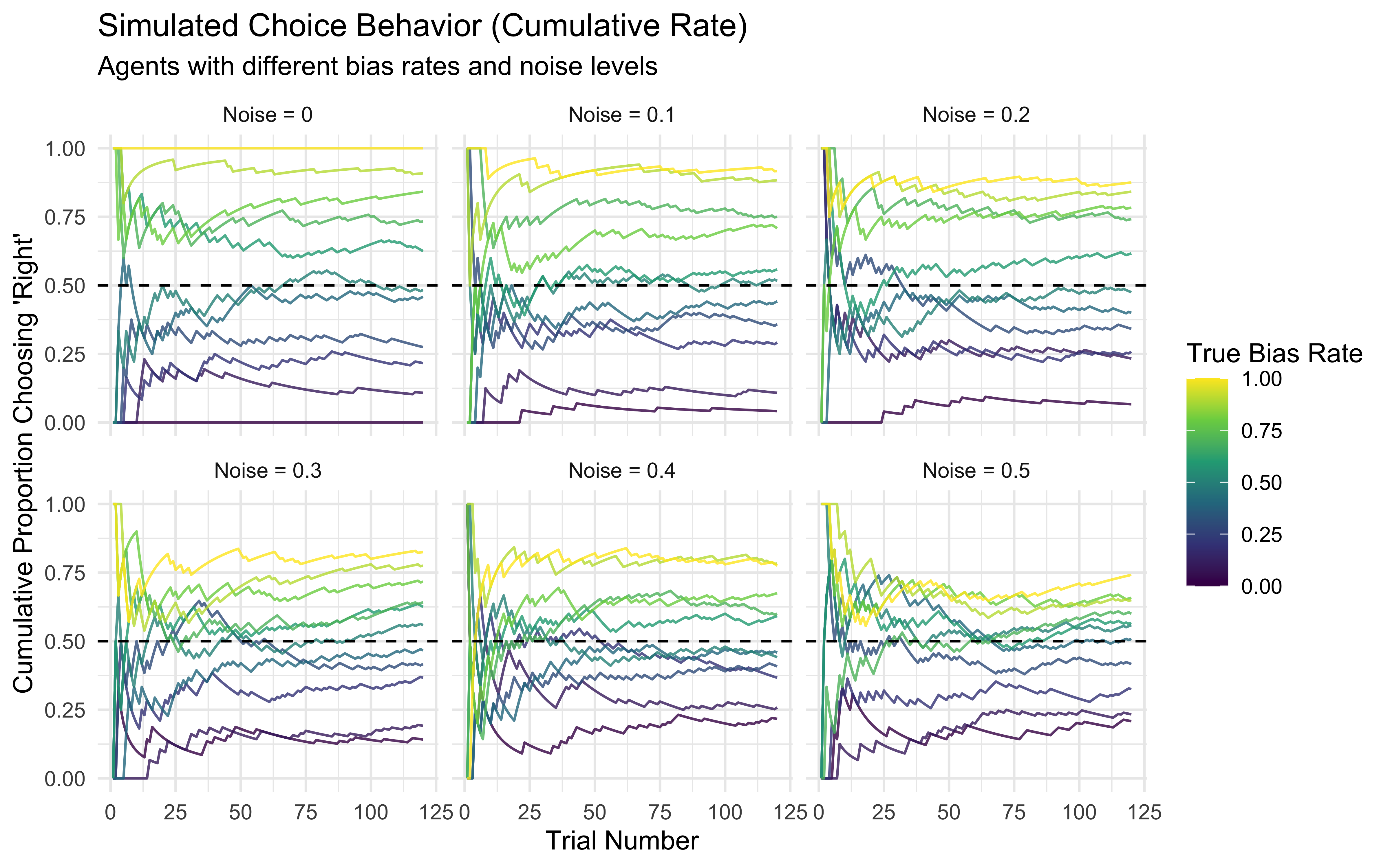
Here we build a new simulation of random agents with bias and noise. The code and visualization is really nothing different from last chapter.
```{r ch05_simulating data}
# Flag to control whether to regenerate simulation/fitting results for the knitted files
# Set to TRUE to rerun everything (takes time!), FALSE to load saved results.
regenerate_simulations <- FALSE

# --- Simulate Data for Fitting ---
# Goal: Generate data from known models/parameters to test our fitting procedures.

trials <- 120 # Number of trials per simulated agent

# Define the agent function (copied from previosu chapter)
# This agent chooses '1' with probability 'rate', potentially adding noise.
RandomAgentNoise_f <- function(rate, noise) {
  # Ensure rate is probability (in case log-odds are passed, though not here)
  rate_prob <- plogis(rate) # Assumes rate might be log-odds; use identity if rate is already probability
  choice <- rbinom(1, 1, rate_prob) # Base choice
  if (noise > 0 & rbinom(1, 1, noise) == 1) { # Check if noise occurs
    choice <- rbinom(1, 1, 0.5) # Override with random 50/50 choice
  }
  return(choice)
}

# --- Generate Data Across Different Conditions ---
# Define relative paths for saving/loading simulation data
sim_data_dir <- "simdata" # Assumes a 'simdata' subdirectory
sim_data_file <- here(sim_data_dir, "ch06_randomnoise.csv")

# Create directory if it doesn't exist
if (!dir.exists(sim_data_dir)) dir.create(sim_data_dir)

if (regenerate_simulations || !file.exists(sim_data_file)) {
  cat("Generating new simulation data...\n")
  # Use expand_grid for cleaner parameter combinations
  param_grid <- expand_grid(
    noise = seq(0, 0.5, 0.1), # Noise levels
    rate = seq(0, 1, 0.1)     # Bias rate levels (probability scale)
  )

  # Use map_dfr for efficient simulation across parameters
  d <- pmap_dfr(param_grid, function(noise, rate) {
    # Simulate choices for one agent/condition
    choices <- map_int(1:trials, ~RandomAgentNoise_f(qlogis(rate), noise)) # Convert rate to log-odds for function if needed
    # Create tibble for this condition
    tibble(
      trial = 1:trials,
      choice = choices,
      true_rate = rate, # Store the true rate used for generation
      true_noise = noise # Store the true noise used
    )
  }) %>%
  # Calculate cumulative rate for visualization
  group_by(true_rate, true_noise) %>%
  mutate(cumulative_rate = cumsum(choice) / row_number()) %>%
  ungroup()

  # Save the generated data
  write_csv(d, sim_data_file)
  cat("Generated new simulation data and saved to", sim_data_file, "\n")
} else {
  # Load existing simulation data
  d <- read_csv(sim_data_file)
  cat("Loaded existing simulation data from", sim_data_file, "\n")
}
# --- Visualize Simulated Data ---
# Plot cumulative rate, faceted by noise level
p1 <- ggplot(d, aes(x = trial, y = cumulative_rate, group = true_rate, color = true_rate)) +
  geom_line(alpha = 0.8) +
  geom_hline(yintercept = 0.5, linetype = "dashed") +
  scale_color_viridis_c() + # Use perceptually uniform color scale
  facet_wrap(~paste("Noise =", true_noise)) + # Facet by noise level
  labs(
    title = "Simulated Choice Behavior (Cumulative Rate)",
    subtitle = "Agents with different bias rates and noise levels",
    x = "Trial Number",
    y = "Cumulative Proportion Choosing 'Right'",
    color = "True Bias Rate"
  ) +
  theme_minimal() +
  ylim(0, 1)

print(p1)
```
## How the Posterior Is Actually Computed
Before we hand this problem to Stan, it is worth understanding what Stan is
actually *doing* — because "posterior ∝ prior × likelihood" is easy to say
and hard to see. This section builds a posterior by hand using a **grid
approximation**: a brute-force method that works when there is only one
parameter and we are willing to evaluate every possible value of it.
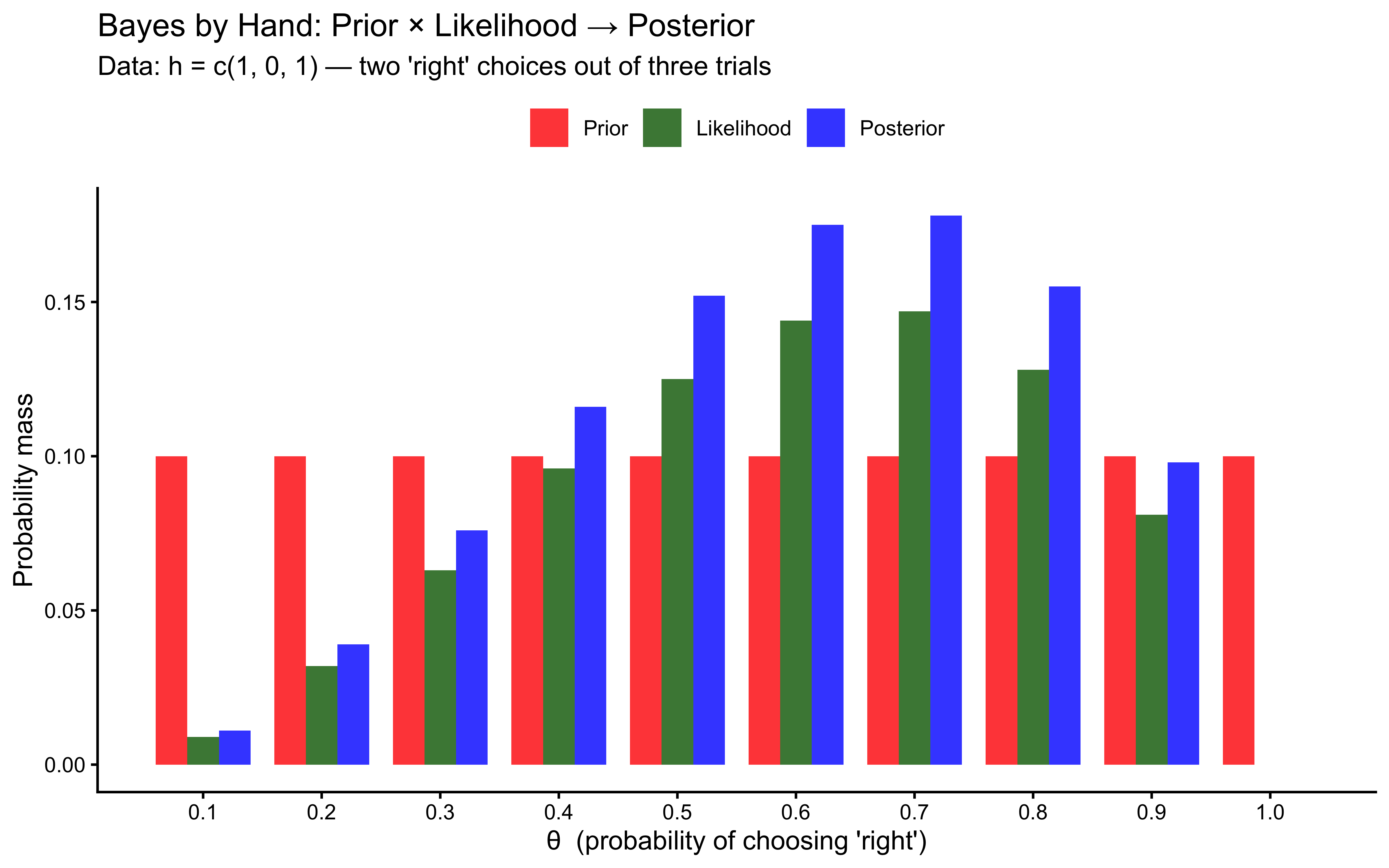
**The setup.** Suppose an agent made 3 choices, picking "right" on trials 1
and 3 and "left" on trial 2 (`h = c(1, 0, 1)`). We want to know: what is
the most plausible value of θ — the agent's underlying bias toward "right"?
**Bayes' rule** tells us:
$$P(\theta \mid \text{data}) \propto P(\theta) \times P(\text{data} \mid \theta)$$
In words: the posterior is proportional to the prior (what we believed before
seeing the data) multiplied by the likelihood (how probable the data is under
each value of θ). We then re-normalize so the result sums to 1.
```{r 04-bayes-by-hand, fig.cap="Grid approximation with 3 observed choices. The posterior (blue) is the pointwise product of the prior (red) and the likelihood (green), re-normalized. Notice that the prior is flat — every value of θ was equally plausible beforehand — and the posterior peaks near θ = 0.7, which best explains seeing 2 'right' choices out of 3."}
# 1. Define a coarse grid of 10 candidate values for theta
theta_grid <- seq(0.1, 1.0, by = 0.1)

# 2. Prior: uniform — Beta(1,1) — every value equally plausible before seeing data
prior <- rep(1, length(theta_grid))
prior <- prior / sum(prior)   # Normalize to sum to 1

# 3. Observed data
h <- c(1, 0, 1)   # 2 "right" out of 3 trials

# 4. Likelihood: P(data | theta)
# Each choice is Bernoulli(theta), so the joint likelihood is the product
# across trials
likelihood <- sapply(theta_grid, function(th) {
  prod(dbinom(h, size = 1, prob = th))
})

# 5. Unnormalized posterior: prior * likelihood (pointwise)
posterior_unnorm <- prior * likelihood

# 6. Normalize so it sums to 1
posterior <- posterior_unnorm / sum(posterior_unnorm)

# --- Display as a table ---
grid_table <- tibble(
  `θ`           = theta_grid,
  `Prior`       = round(prior, 3),
  `Likelihood`  = round(likelihood, 4),
  `Posterior`   = round(posterior, 3)
)

knitr::kable(grid_table,
             caption = "Grid approximation: prior × likelihood → posterior (3 observations)")
# --- Plot all three distributions ---
grid_long <- grid_table %>%
  rename(theta = `θ`, prior = Prior, likelihood = Likelihood, posterior = Posterior) %>%
  pivot_longer(c(prior, likelihood, posterior),
               names_to = "distribution", values_to = "mass") %>%
  mutate(distribution = factor(distribution,
                                levels = c("prior", "likelihood", "posterior"),
                                labels = c("Prior", "Likelihood", "Posterior")))

ggplot(grid_long, aes(x = theta, y = mass, fill = distribution)) +
  geom_col(position = "dodge", alpha = 0.8, width = 0.08) +
  scale_fill_manual(values = c("Prior" = "red", "Likelihood" = "darkgreen",
                                "Posterior" = "blue")) +
  scale_x_continuous(breaks = theta_grid) +
  labs(
    title    = "Bayes by Hand: Prior × Likelihood → Posterior",
    subtitle = "Data: h = c(1, 0, 1) — two 'right' choices out of three trials",
    x        = "θ  (probability of choosing 'right')",
    y        = "Probability mass",
    fill     = NULL
  ) +
  theme_classic() +
  theme(legend.position = "top")
```
Three things to notice from the table and the plot:
1. **The prior is flat.** Before seeing any data, every value of θ is equally
plausible. This is what `Beta(1, 1)` means — maximal prior ignorance.
2. **The likelihood peaks near θ = 0.7.** The agent chose "right" 2 out of
3 times, so θ = 0.7 makes the observed sequence most probable. Values near
0 or 1 make it very improbable.
3. **The posterior is the pointwise product, re-normalized.** It is narrower
than the prior (the data ruled out extreme values) and centred on the
likelihood peak. This is exactly the "update": the data shifted our beliefs
from flat to concentrated.
**Why Stan instead of a grid?** This worked with 1 parameter and 10 grid
points. With 2 parameters and 100 grid points each, we need 100 × 100 = 10,000
evaluations. With 5 parameters: 100⁵ = **10 billion**. The grid grows
exponentially — this is the *curse of dimensionality*. Stan's Hamiltonian
Monte Carlo (HMC) sampler sidesteps this by *sampling* from regions of high
posterior probability rather than evaluating every possible combination. The
samples it returns are the blue histogram you will see in the next section —
same idea, just no grid required.
## Building our First Stan Model: Inferring Bias Rate
N.B. Refer to the video and slides for the step by step build-up of the Stan code.
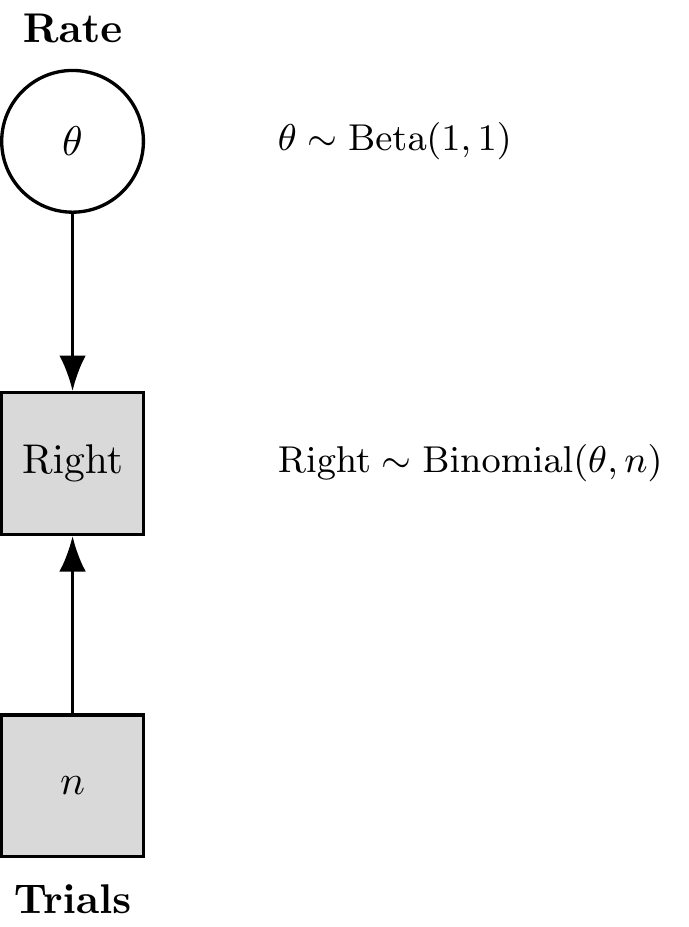
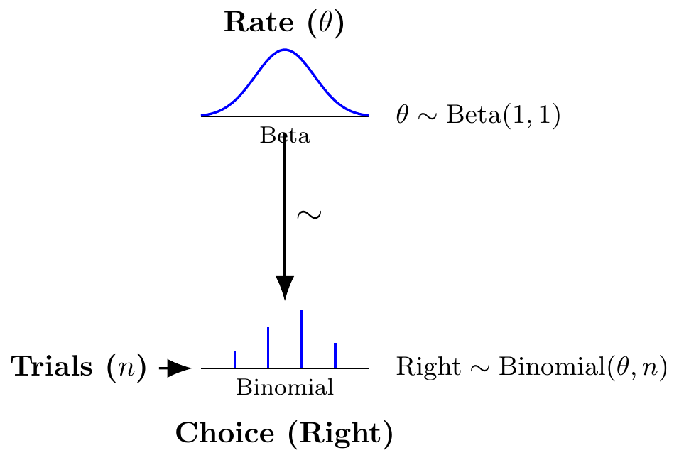
Let's use Stan to estimate the underlying bias `rate` (which we'll call `theta` in the model) from just the sequence of choices (`h`) generated by one of our simulated agents. This model is represented in the
```{tikz, echo=FALSE, fig.cap="Binomial Model with Formulas", fig.ext = 'png', cache=TRUE}
\usetikzlibrary{positioning, shapes.geometric, arrows.meta}
\begin{tikzpicture}[
% GLOBAL STYLES
node distance=1.5cm,
continuous/.style={circle, draw=black, thick, minimum size=1.2cm},
discrete/.style={rectangle, draw=black, thick, minimum size=1.2cm},
observed/.style={fill=gray!30},
latent/.style={fill=white},
stochastic/.style={->, >={Latex[length=3mm]}, thick},
% New style for the formula text
formula/.style={right=1cm, align=left, font=\small}
]
% --- NODES ---
% 1. Rate (Theta) - Top
\node[continuous, latent] (theta) {$\theta$};
% 2. Right (k) - Middle
\node[discrete, observed, below=of theta] (k) {Right};
% 3. Trials (n) - Bottom
\node[discrete, observed, below=of k] (n) {$n$};
% --- EDGES ---
\draw[stochastic] (theta) -- (k);
\draw[stochastic] (n) -- (k);
% --- FORMULAS (The new part) ---
% Formula for Theta
% We use 'align=left' to allow multiple lines if you want to list options
\node[formula] at (theta.east) {
$\theta \sim \text{Beta}(1,1)$
};
% Formula for Right (Outcome)
% Note: If you have 'n' trials, the distribution is usually Binomial
\node[formula] at (k.east) {
$\text{Right} \sim \text{Binomial}(\theta, n)$
};
% (Optional) Label for N if it's fixed
% \node[formula] at (n.east) { $n = 100$ };
% --- LABELS ---
\node[above=0.1cm of theta] {\textbf{Rate}};
\node[below=0.1cm of n] {\textbf{Trials}};
\end{tikzpicture}
```
```{tikz, echo=FALSE, fig.cap="Kruschke-Style Binomial Model", fig.ext = 'png', cache=TRUE}
\usetikzlibrary{positioning, arrows.meta, calc, shapes.geometric}
\begin{tikzpicture}[
node distance=2.5cm,
% 1. DEFINE THE ICONS (PICS)
% Beta Distribution Icon (Smooth Curve)
pics/beta_dist/.style={
code={
% Axis
\draw[thin] (-1,0) -- (1,0);
% Curve (Beta-like hump)
\draw[thick, blue] plot[domain=-1:1, samples=50] (\x, {0.8*exp(-4*\x*\x)});
% Label inside or near
\node[font=\footnotesize, below] at (0,0) {Beta};
}
},
% Binomial Distribution Icon (Bar Chart)
pics/binom_dist/.style={
code={
% Axis
\draw[thin] (-1,0) -- (1,0);
% Bars
\draw[thick, blue, ycomb] plot coordinates {
(-0.6, 0.2) (-0.2, 0.5) (0.2, 0.7) (0.6, 0.3)
};
% Label
\node[font=\footnotesize, below] at (0,0) {Binomial};
}
},
% Arrow Style with Tilde
stochastic/.style={->, >={Latex[length=3mm]}, thick, font=\large},
label_text/.style={align=center, font=\small}
]
% --- TOP: PRIOR (RATE) ---
% We define a coordinate for the center of the Beta plot
\coordinate (prior_pos) at (0,0);
% Draw the picture
\draw (prior_pos) pic (beta) {beta_dist};
% Add Labels for Prior
\node[above=0.8cm of prior_pos, font=\bfseries] {Rate ($\theta$)};
\node[right=1.2cm of prior_pos, anchor=west, font=\small] {$\theta \sim \text{Beta}(1,1)$};
% --- BOTTOM: LIKELIHOOD (CHOICE) ---
% Position it below
\coordinate[below=3cm of prior_pos] (like_pos);
% Draw the picture
\draw (like_pos) pic (binom) {binom_dist};
% Add Labels for Likelihood
\node[below=0.5cm of like_pos, font=\bfseries] {Choice (Right)};
\node[right=1.2cm of like_pos, anchor=west, font=\small] {$\text{Right} \sim \text{Binomial}(\theta, n)$};
% --- SIDE: TRIALS (n) ---
% Just a text node feeding in
\node[left=1.5cm of like_pos, font=\bfseries] (n) {Trials ($n$)};
% --- EDGES ---
% 1. From Beta to Binomial (Stochastic)
% We start the arrow slightly below the top axis and end slightly above the bottom one
\draw[stochastic] (0, -0.2) -- (0, -2.2) node[midway, right] {$\sim$};
% 2. From Trials to Binomial (Deterministic/Parameter)
\draw[stochastic] (n) -- (-1.1, -3); % Connects to the side of the plot area
\end{tikzpicture}
```
We'll start with a simple case: an agent with `rate = 0.8` and `noise = 0`.
**Preparing Data for Stan**
Why a list? Well, dataframes (now tibbles) are amazing. But they have a big drawback: they require each variable to have the same length. Lists do not have that limitation, they are more flexible. So, lists. We'll have to learn how to live with them.
```{r 04-prep-stan-data}
# Subset data for one specific agent simulation (rate=0.8, noise=0)
d1 <- d %>% filter(true_rate == 0.8, true_noise == 0.0) # Make sure noise level matches

# Stan requires data in a list format
data_for_stan <- list(
  n = trials,     # Number of trials (integer)
  h = d1$choice   # Vector of choices (0s and 1s) for this agent
)

str(data_for_stan) # Show the structure of the list
```
### Model
We write the stan code within the R code (so I can show it to you more easily), then we save it as a stan file, which can be loaded at a later stage in order to compile it. [Missing: more info on compiling etc.]
Remember that the minimal Stan model requires 3 chunks, one specifying the data it will need as input; one specifying the parameters to be estimated; one specifying the model within which the parameters appear, and the priors for those parameters.
```{r ch05_defining the biased model}
# This R chunk defines the Stan code as a string and writes it to a file.
# It's marked eval=FALSE because we don't run the R code defining the string here,
# but the Stan code itself IS the important content.

stan_model_code <- "
// Stan Model: Simple Bernoulli for Bias Estimation
// Goal: Estimate the underlying probability (theta) of choosing 1 ('right')
//       given a sequence of binary choices.

// 1. Data Block: Declares the data Stan expects from R
data {
  int<lower=1> n;        // Number of trials (must be at least 1)
  array[n] int<lower=0, upper=1> h; // Array 'h' of length 'n' containing choices (0 or 1)
}

// 2. Parameters Block: Declares the parameters the model will estimate
parameters {
  real<lower=0, upper=1> theta; // The bias parameter (probability), constrained between 0 and 1
}

// 3. Model Block: Defines the priors and the data model (used as likelihood during inference)
model {
  // Prior: Our belief about theta *before* seeing the data.
  // We use a Beta(1, 1) prior, which is equivalent to a Uniform(0, 1) distribution.
  // This represents maximal prior ignorance about the bias.
  // 'target +=' adds the log-probability density to the overall model log-probability.
  target += beta_lpdf(theta | 1, 1); // lpdf = log probability density function

  // Likelihood: How the data 'h' depend on the parameter 'theta'.
  // We model each choice 'h' as a Bernoulli trial with success probability 'theta'.
  // The model assesses how likely the observed sequence 'h' is given a value of 'theta'.
  target += bernoulli_lpmf(h | theta); // lpmf = log probability mass function (for discrete data)
}

// 4. Generated Quantities Block (Optional but useful)
// Code here is executed *after* sampling, using the estimated parameter values.
// Useful for calculating derived quantities or predictions.
generated quantities {
  // let's generate the prior for visualization
  // first we define it
  real<lower = 0, upper = 1> prior_theta;
  // then we generate it
  prior_theta = beta_rng(1, 1); // Draw a random sample from the prior distribution for theta
}
"
# Define relative path for Stan model file
stan_model_dir <- "stan"
stan_file_bernoulli <- here(stan_model_dir, "ch06_SimpleBernoulli.stan")

# Create directory if needed
if (!dir.exists(stan_model_dir)) dir.create(stan_model_dir)

# Write the Stan code to the file
writeLines(stan_model_code, stan_file_bernoulli)

cat("Stan model written to:", stan_file_bernoulli, "\n")
```
Compiling and Fitting the Stan Model
Now we use cmdstanr to compile this model (translating it into efficient C++ code) and then run the MCMC sampler to get posterior estimates for theta.
```{r 04 fit the biased model}
## --- Compile and Fit ---
# Specify model file path
stan_file_bernoulli <- here("stan", "ch06_SimpleBernoulli.stan")
# Define path for saving fitted model object
stan_results_dir <- "simmodels"
model_file_bernoulli <- here(stan_results_dir, "ch06_SimpleBernoulli.rds")

if (!dir.exists(stan_results_dir)) dir.create(stan_results_dir)

if (regenerate_simulations || !file.exists(model_file_bernoulli)) {
  cat("Compiling and fitting Stan model (Bernoulli)...\n")
  # Compile the Stan model (only needs to be done once unless code changes)
  mod_bernoulli <- cmdstan_model(stan_file_bernoulli,
                                 cpp_options = list(stan_threads = FALSE), # Enable threading
                                 stanc_options = list("O1")) # Basic optimization

  # Sample from the posterior distribution using MCMC
  fit_bernoulli <- mod_bernoulli$sample(
    data = data_for_stan,          # The data list we prepared
    seed = 123,                    # For reproducible MCMC sampling
    chains = 4,                    # Number of parallel Markov chains (recommend 4)
    parallel_chains = 4, # Run chains in parallel
    #threads_per_chain = 1,         # For within-chain parallelization (usually 1 is fine)
    iter_warmup = 1000,            # Number of warmup iterations per chain (discarded)
    iter_sampling = 2000,          # Number of sampling iterations per chain (kept)
    refresh = 0,                   # How often to print progress updates. 0 means never since the model is so fast
    max_treedepth = 10,            # Controls complexity of MCMC steps (adjust if needed)
    adapt_delta = 0.8              # Target acceptance rate (adjust if divergences occur)
  )

  # Save the fitted model object
  fit_bernoulli$save_object(file = model_file_bernoulli)
  cat("Model fit completed and saved to:", model_file_bernoulli, "\n")
} else {
  # Load existing fitted model object
  fit_bernoulli <- readRDS(model_file_bernoulli)
  cat("Loaded existing model fit from:", model_file_bernoulli, "\n")
}
```
### Assessing MCMC Health (The Mandatory Diagnostics)
> *Why check diagnostics before looking at the estimates?* The posterior
> distribution Stan returns is only valid if the sampler explored the parameter
> space correctly. If it did not — due to divergent transitions, poor mixing, or
> insufficient samples — the numbers in the posterior are artifacts of the
> algorithm, not properties of the model. Looking at estimates from a broken
> sampler is like reading a map drawn by a robot that kept falling over: the map
> looks plausible but cannot be trusted. Diagnostics are the check that the robot
> walked properly before you navigate with its map.
Before we look at the parameter estimates, we MUST check whether the model was able to sample the posterior space: the health of the MCMC chains. Fitting a model is like sending a robotic explorer (the sampler) to map a landscape (the posterior). If the robot's tracks are broken, the map is mathematically invalid. We must check:
1. **Divergences:** Did the simulation crash? (Zero tolerance).
2. **$\hat{R}$ (R-hat):** Did our 4 independent chains map the exact same space? (Must be strictly $< 1.01$).
3. **Effective Sample Size (ESS):** Do we have enough *truly independent* draws? (Bulk and Tail ESS should be $> 400$).
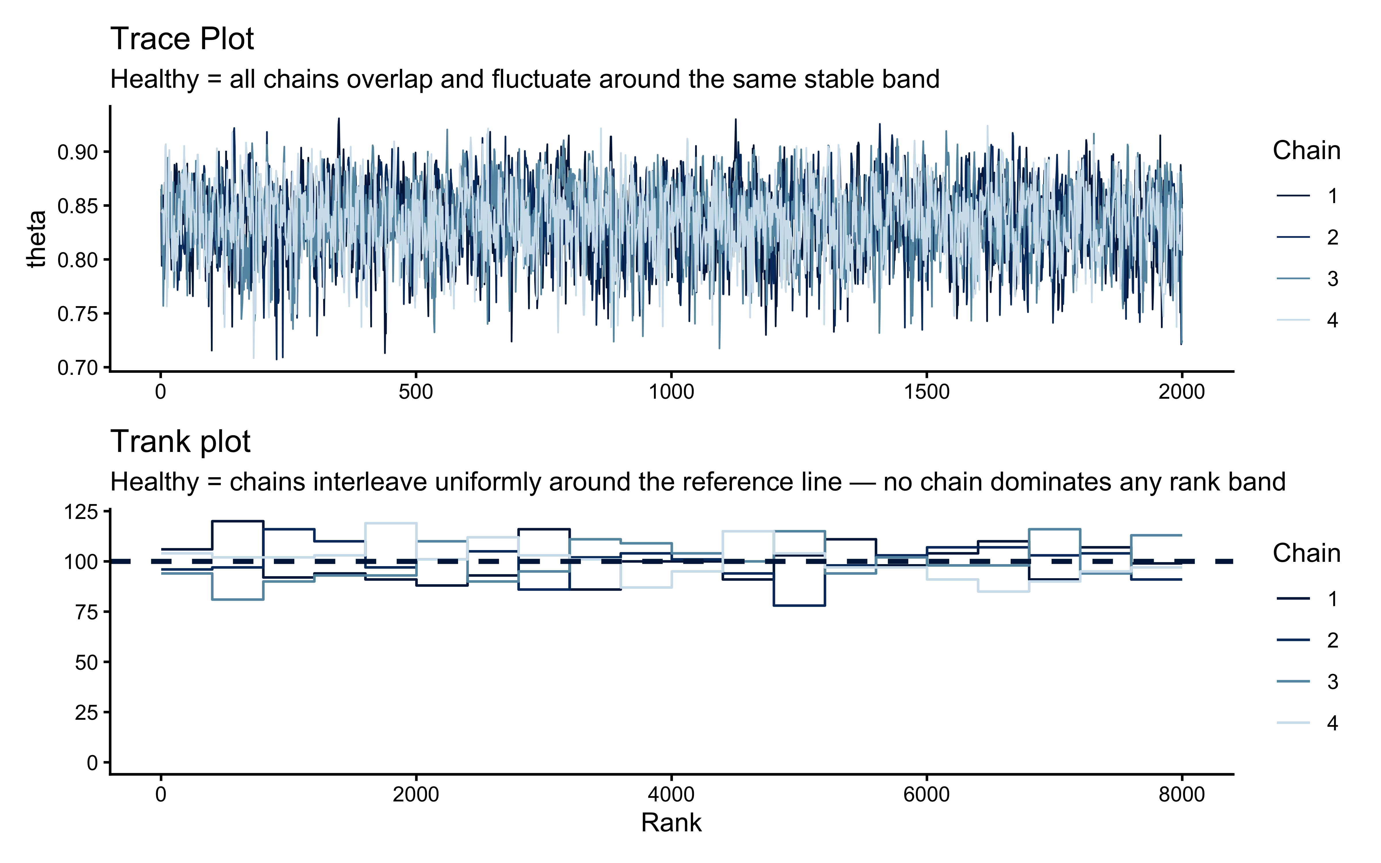
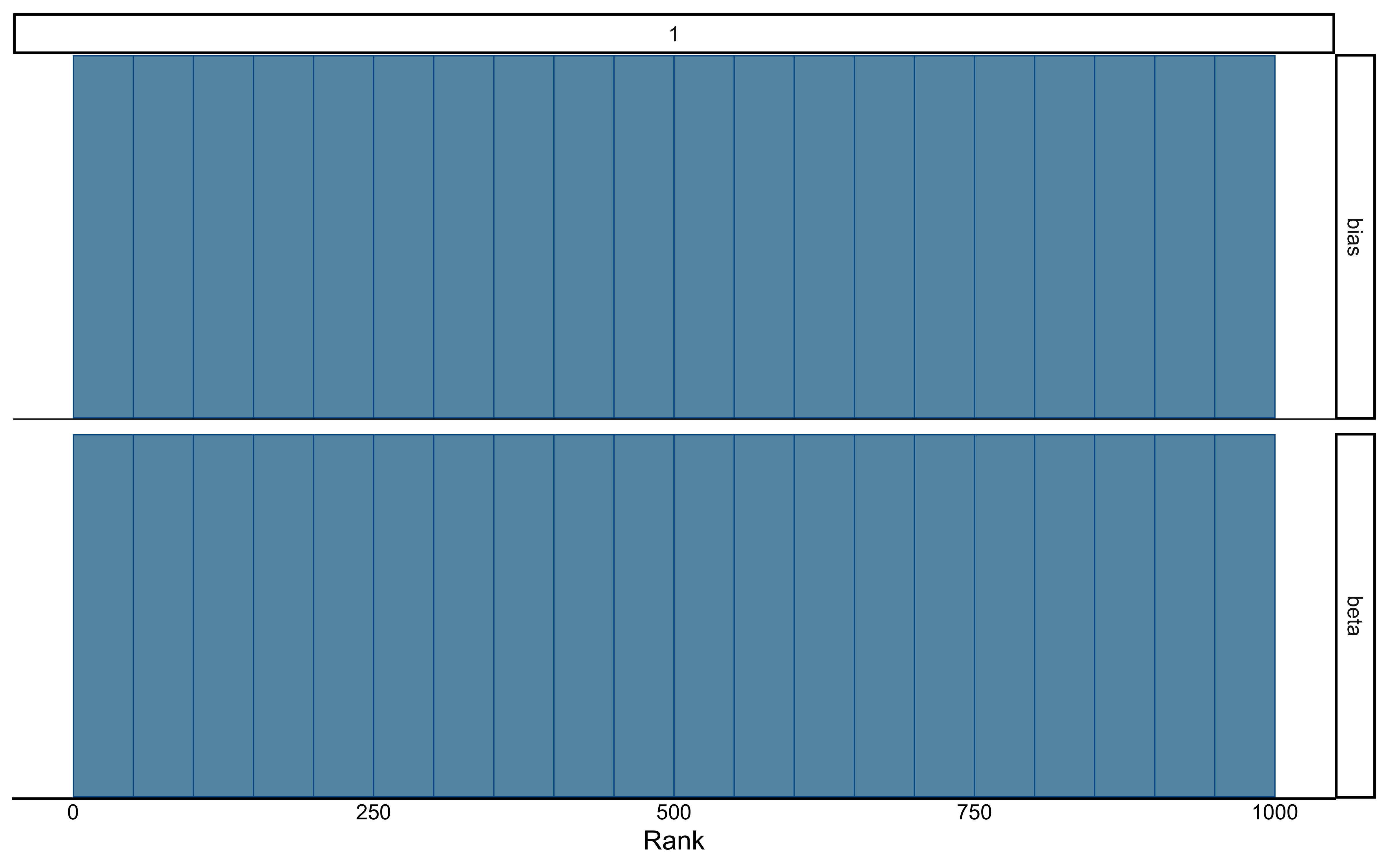
4. **Visual Diagnostics:** Trace plots (should look like a "hairy caterpillar") and Rank Histograms (should be uniform across chains).
Let's run this mandatory diagnostic battery on our first fit:
```{r 04 biased model quality}
# 1. Check for Divergent Transitions
diagnostics <- fit_bernoulli$diagnostic_summary()
cat("Divergent transitions per chain:", paste(diagnostics$num_divergent, collapse = ", "), "\n")
# 2. Check R-hat and ESS metrics
fit_summary <- fit_bernoulli$summary(variables = "theta")
print(fit_summary %>% dplyr::select(variable, mean, rhat, ess_bulk, ess_tail))
# 3. Visual Checks (Trace and Rank Plots)
draws_df <- as_draws_df(fit_bernoulli$draws())

# A healthy trace plot is well-mixed with no wandering
p_trace <- mcmc_trace(draws_df, pars = "theta") +
  theme_classic() +
  ggtitle("Trace Plot",
          subtitle = "Healthy = all chains overlap and fluctuate around the same stable band")

# A healthy rank histogram has uniform bars across all chains
p_rank <- mcmc_rank_overlay(draws_df, pars = "theta", ref_line = TRUE) +
  theme_classic() +
  ggtitle("Trank plot", subtitle = "Healthy = chains interleave uniformly around the reference line — no chain dominates any rank band")

p_trace / p_rank
# 4. Look at the Posterior Estimate
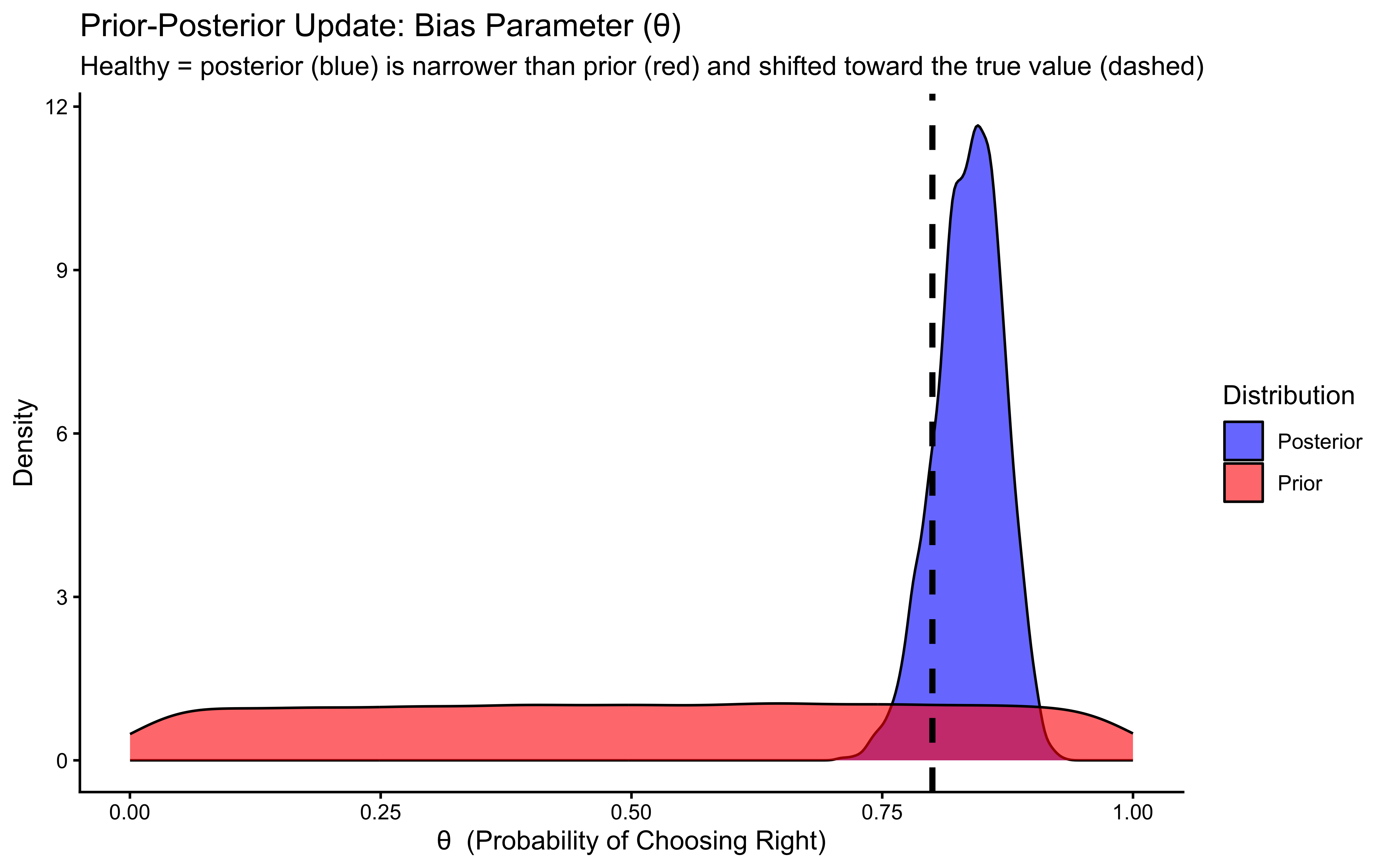
ggplot(draws_df) +
geom_density(aes(theta, fill = "Posterior"), alpha = 0.6) +
geom_density(aes(prior_theta, fill = "Prior"), alpha = 0.6) +
geom_vline(xintercept = 0.8, linetype = "dashed", color = "black", linewidth = 1.2) +
scale_fill_manual(values = c("Posterior" = "blue", "Prior" = "red")) +
labs(
title = "Prior-Posterior Update: Bias Parameter (θ)",
subtitle = "Healthy = posterior (blue) is narrower than prior (red) and shifted toward the true value (dashed)",
x = "θ (Probability of Choosing Right)",
y = "Density",
fill = "Distribution"
) +
theme_classic()
```
The posterior (blue) is substantially narrower than the prior (red) and has shifted toward the true value of 0.8 (dashed line). The posterior mean is approximately 0.755, not exactly 0.8 — this is expected with only 120 trials and is not a sign that something is wrong. What matters is that (a) the posterior is much more informative than the prior, confirming the data were indeed informative, and (b) the true value 0.8 sits comfortably within the credible interval. If the posterior were identical to the prior, the data would be telling us nothing; if the posterior were centered far from the true value and excluded it, the model would be misspecified.
Now we build the same model, but using the log odds scale for the theta parameter, which will become useful later when we condition theta on variables and build multilevel models (as we can do what we want in a log odds space and it will always be bound between 0 and 1).
**Alternative Parameterization: Log-Odds Scale**
While estimating theta directly as a probability (0-1) is intuitive, it can sometimes be computationally advantageous or necessary for more complex models (like multilevel models in a later chapter) to estimate parameters on an unbounded scale.
The logit (log-odds) transformation converts a probability $p$ (from 0 to 1) to log-odds (from $-\infty$ to $+\infty$): $$\text{logit}(p) = \log\left(\frac{p}{1-p}\right)$$
The inverse transformation (logistic function or inv_logit) converts log-odds back to probability: $$\text{inv\_logit}(x) = \frac{1}{1 + \exp(-x)}$$
We can rewrite our Stan model to estimate theta on the log-odds scale. However, we must be careful with our priors, as the non-linear transformation distorts the probability mass.
* Too Narrow: A standard normal prior $\lambda \sim \text{Normal}(0, 1)$ concentrates mass around $p=0.5$, biasing the model toward chance.
* Too Wide: A wide prior (e.g., $\lambda \sim \text{Normal}(0, 5)$) pushes mass to the extremes (0 and 1), implying we expect deterministic behavior.
* Just Right: To approximate a uniform distribution on the probability scale (like our Beta(1,1)), we typically use $\lambda \sim \text{Normal}(0, 1.5)$. This is the specific "sweet spot" that is essentially flat, avoiding both the center-bias of narrow priors and the extreme-bias of wide priors.
```{r 04-define-stan-model-logit}
# Stan code using logit parameterization
stan_model_logit_code <- "
// Stan Model: Simple Bernoulli (Logit Parameterization)
// Estimate theta on the log-odds scale

data {
  int<lower=1> n;
  array[n] int<lower=0, upper=1> h;
}

parameters {
  real theta_logit; // Parameter is now on the unbounded log-odds scale
}

model {
  // Prior on log-odds scale (e.g., Normal(0, 1.5))
  // Normal(0, 1.5) on log-odds corresponds roughly to a diffuse prior on probability scale
  target += normal_lpdf(theta_logit | 0, 1.5);

  // Likelihood using the logit version of the Bernoulli PMF
  // This tells Stan that theta_logit is on the log-odds scale
  target += bernoulli_logit_lpmf(h | theta_logit);
}

generated quantities {
  // Generate the prior for viz purposes
  real prior_theta = inv_logit(normal_rng(0, 1.5)); // Sample from the log-odds prior
  // Convert estimate back to probability scale for easier interpretation
  real<lower=0, upper=1> theta = inv_logit(theta_logit);
}
"
# Define file path
stan_file_logit <- here(stan_model_dir, "ch06_SimpleBernoulli_logodds.stan")
# Write the Stan code to the file
writeLines(stan_model_logit_code, stan_file_logit)
cat("Stan model (logit) written to:", stan_file_logit, "\n")
```
::: {.callout-tip title="Stan Efficiency — Sufficient Statistics: Aggregate IID Trials"}
When all trials are **independently and identically distributed** (no memory, no sequential
dependency, one $\theta$ for the whole session), you can replace a loop of $N$ Bernoulli calls
with a single Binomial call on the **sufficient statistic** — the total number of successes.
```stan
// Slower: N separate Bernoulli evaluations (one autodiff node each)
for (i in 1:N)
  target += bernoulli_logit_lpmf(h[i] | theta_logit);

// Faster: one Binomial evaluation — mathematically identical for IID data
target += binomial_logit_lpmf(sum(h) | N, theta_logit);
```
Pass `sum(h)` and `N` as integers rather than the full array — Stan never sees the
individual trial values.
**When this applies:** single-subject models with one rate parameter per session (Chapters 4–5).
**When it does not apply:** any model where the likelihood varies by trial — memory
models, multilevel models with per-subject parameters indexed by `subj_id`, sequential
belief-updating models. For those, the per-trial loop is necessary.
:::
```{r ch04_fit_logit_model}
## With the logit format
## Specify where the model is
file <- here("stan", "ch06_SimpleBernoulli_logodds.stan")

# File path for saved model
model_file <- here("simmodels","ch06_SimpleBernoulli_logodds.rds")

# Check if we need to rerun the simulation
if (regenerate_simulations || !file.exists(model_file)) {
  # Compile the model
  mod <- cmdstan_model(file,
                       cpp_options = list(stan_threads = FALSE),
                       stanc_options = list("O1"))

  # The following command calls Stan with specific options.
  samples_biased_logodds <- mod$sample(
    data = data_for_stan,
    seed = 123,
    chains = 2,
    parallel_chains = 2,
    #threads_per_chain = 1,
    iter_warmup = 1000,
    iter_sampling = 2000,
    refresh = 0,
    max_treedepth = 20,
    adapt_delta = 0.99,
  )

  # Save the fitted model
  samples_biased_logodds$save_object(file = model_file)
  cat("Generated new model fit and saved to", model_file, "\n")
} else {
  # Load existing results
  cat("Loading biased model (log-odds) samples...\n")
  samples_biased_logodds <- readRDS(model_file)
  cat("Available parameters:", paste(colnames(as_draws_df(samples_biased_logodds$draws())), collapse = ", "), "\n")
  cat("Loaded existing model fit from", model_file, "\n")
}
```
### Summarizing the results
```{r 04 biased model log-odds quality assessment}
# Summary
samples_biased_logodds$summary()
# Extract posterior samples and include sampling of the prior:
draws_df_biased_logodds <- as_draws_df(samples_biased_logodds$draws())

# Explicitly extract theta parameter
theta_param_logodds <- draws_df_biased_logodds$theta
cat("Successfully extracted theta parameter with", length(theta_param_logodds), "values\n")
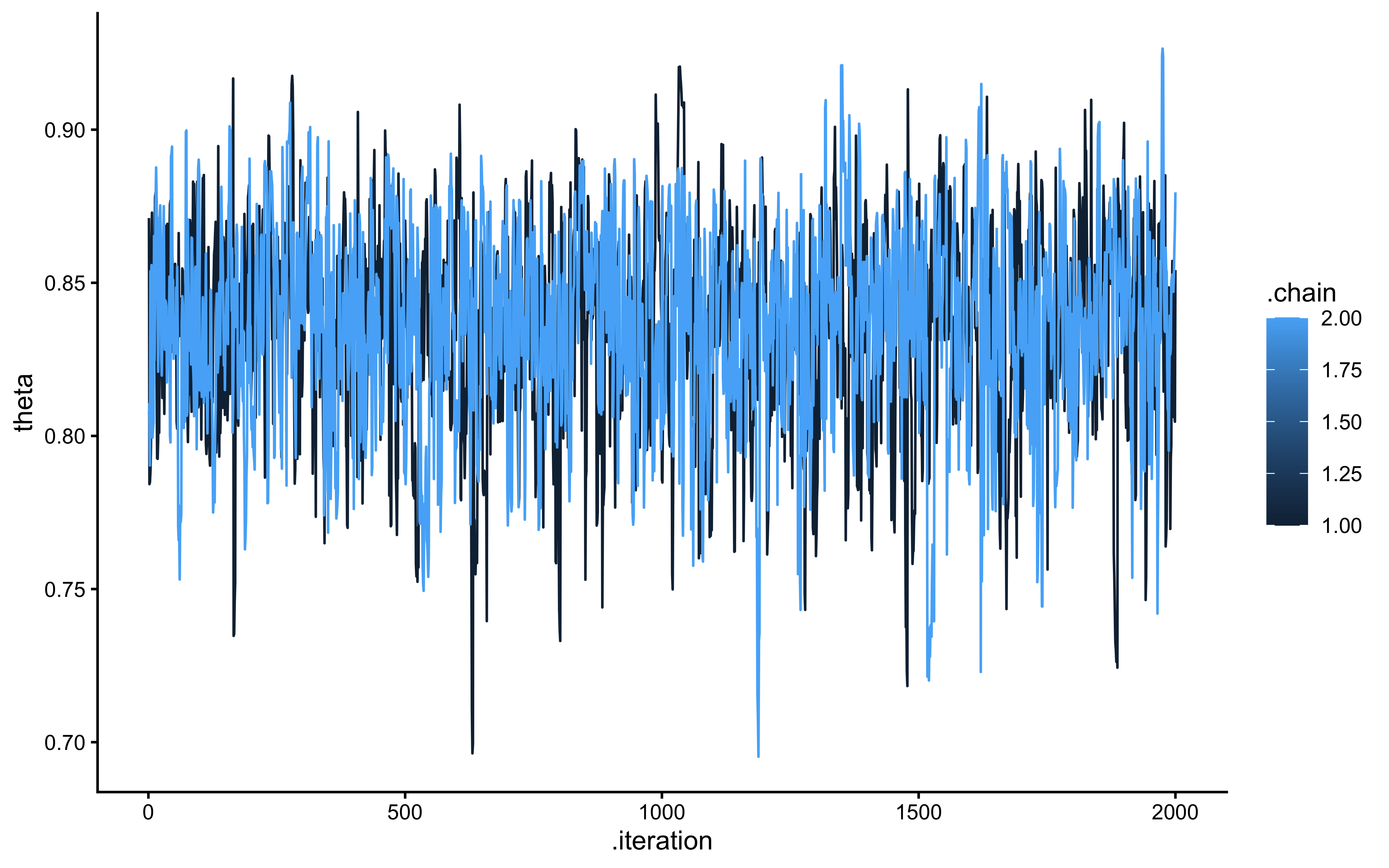
ggplot(draws_df_biased_logodds, aes(.iteration, theta, group = .chain, color = .chain)) +
  geom_line() +
  theme_classic()
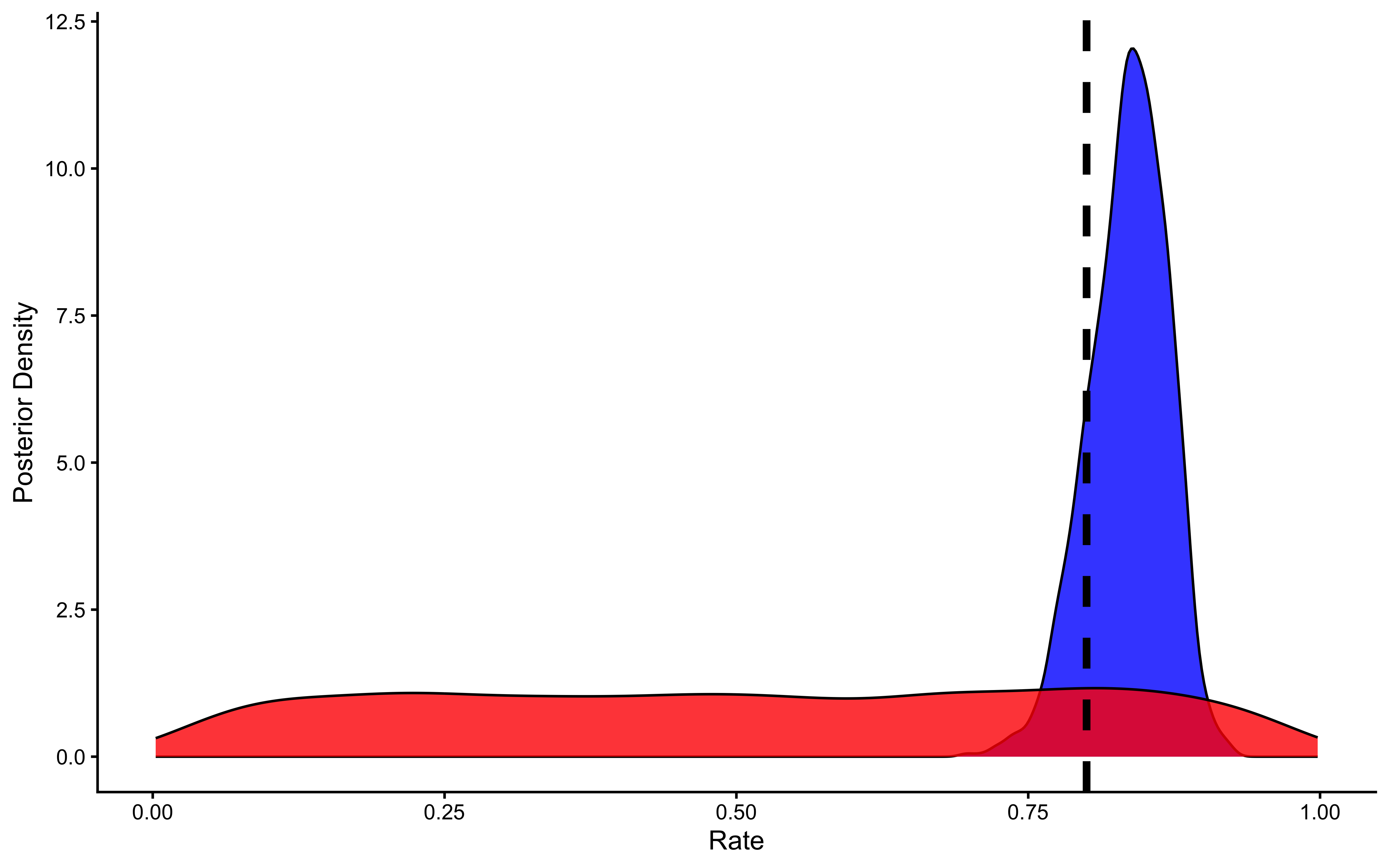
# Now let's plot the density for theta (prior and posterior)
ggplot(draws_df_biased_logodds) +
  geom_density(aes(theta), fill = "blue", alpha = 0.8) +
  geom_density(aes(prior_theta), fill = "red", alpha = 0.8) +
  geom_vline(xintercept = 0.8, linetype = "dashed", color = "black", size = 1.5) +
  xlab("Rate") +
  ylab("Posterior Density") +
  theme_classic()
```
We can see that the results are very similar.
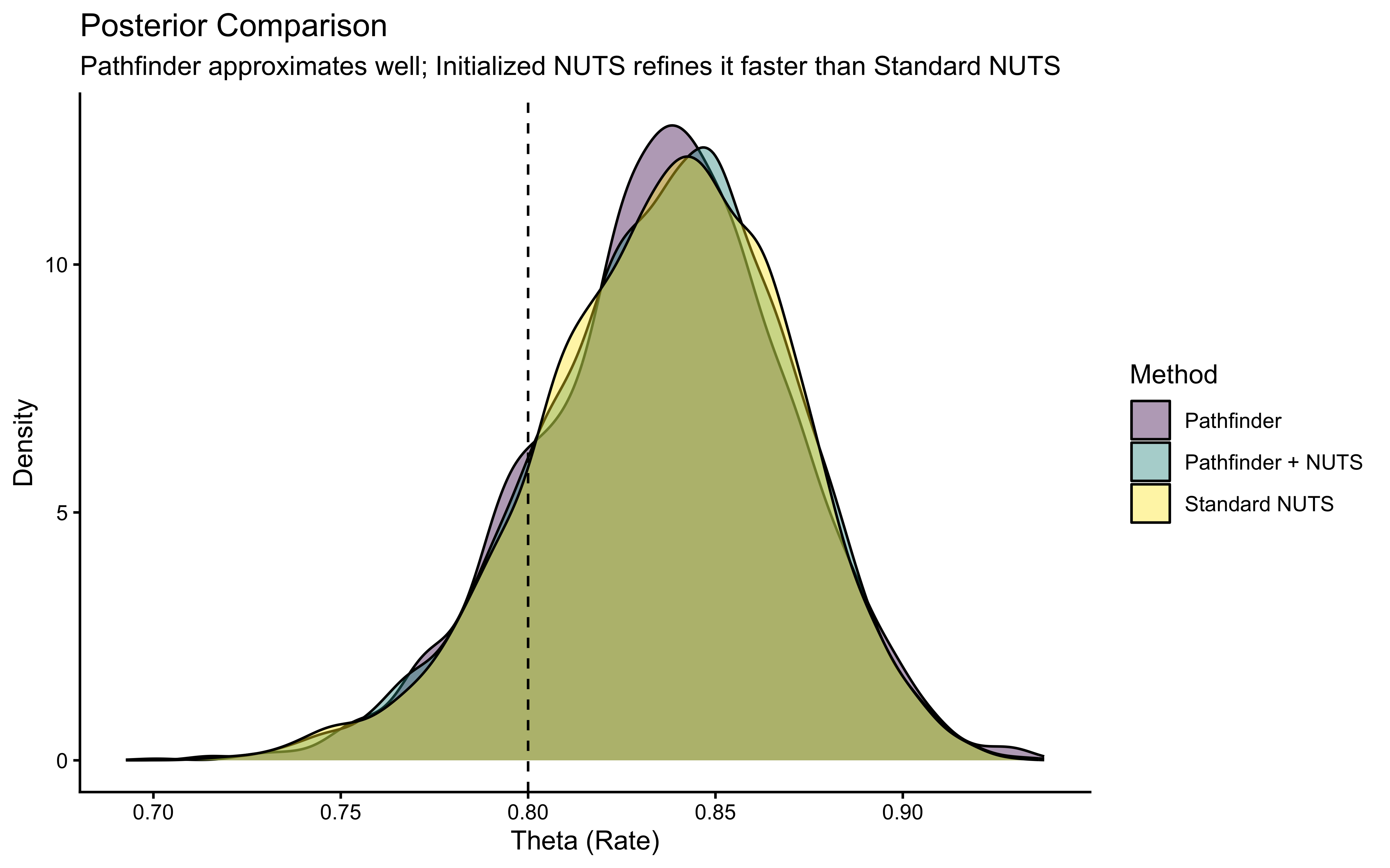
## Bonus: Pathfinder Variational Inference vs. Full MCMC
::: {.callout-tip title="Stan Optimization: Pathfinder as Warm-Start Initialization"}
Stan's default NUTS-HMC sampler draws posterior samples by simulating a Hamiltonian dynamical system. During **warm-up**, the sampler adapts its step size and metric — a phase that can take hundreds of iterations if chains start far from the posterior mass. **Pathfinder** [@zhang2022pathfinder] is a fast variational approximation that traces the L-BFGS optimization path from an initial point to the posterior mode and fits a series of multivariate normal approximations along the way. It is not a gold-standard posterior, but it tells HMC *roughly where the posterior lives* before NUTS begins.
Three strategies, in order of increasing accuracy and cost:
| Strategy | When to use | Typical speed |
|---|---|---|
| **Pathfinder alone** | Quick exploration, prior sensitivity checks | ~10–50× faster than NUTS |
| **NUTS with default init** | Standard analysis | Baseline |
| **Pathfinder → NUTS warm-start** | Hierarchical or complex models where warm-up is slow | 20–60% faster than default NUTS |
The warm-start trick: run `mod$pathfinder(...)` to get a posterior approximation, then pass it as `init` to `mod$sample(...)`. This replaces the random Uniform(−2, 2) starting points with draws from the Pathfinder approximation, letting the sampler skip most of the warm-up trajectory. We will use this pattern throughout the book for models with challenging geometry or many parameters.
**When Pathfinder fails:** Near-degenerate posteriors (e.g., hard funnels, flat ridges) can cause Pathfinder's variational approximation to collapse. Always wrap it in `tryCatch(..., error = function(e) NULL)` and fall back to explicit per-chain inits centered on prior medians if it returns `NULL`.
:::
```{r ch05_intro to pathfinded}
## Bonus content: Benchmarking NUTS, Pathfinder, and Pathfinder-initialized NUTS

# We will compare three methods:
# 1. Standard NUTS (MCMC)
# 2. Pathfinder (Variational Inference)
# 3. NUTS initialized with Pathfinder

# Define file paths for all three models
file_nuts_std  <- here("simmodels", "ch06_benchmark_nuts_std.rds")
file_pathfinder <- here("simmodels", "ch06_benchmark_pathfinder.rds")
file_nuts_init  <- here("simmodels", "ch06_benchmark_nuts_init.rds")

stan_file_logit <- here::here("stan", "ch06_SimpleBernoulli_logodds.stan")
mod <- cmdstan_model(
  stan_file_logit,
  cpp_options = list(stan_threads = FALSE),
  stanc_options = list("O1")
)

# --- 1. Run Standard NUTS (Baseline) ---
if (regenerate_simulations || !file.exists(file_nuts_std)) {
  cat("Running Standard NUTS...\n")
  fit_nuts_std <- mod$sample(
    data = data_for_stan,
    seed = 123,
    chains = 4,
    parallel_chains = 4,
    iter_warmup = 1000, # Standard warmup
    iter_sampling = 2000,
    refresh = 0
  )
  fit_nuts_std$save_object(file_nuts_std)
} else {
  fit_nuts_std <- readRDS(file_nuts_std)
}

# --- 2. Run Pathfinder ---
if (regenerate_simulations || !file.exists(file_pathfinder)) {
  cat("Running Pathfinder...\n")
  fit_pathfinder <- mod$pathfinder(
    data = data_for_stan,
    seed = 123,
    draws = 4000,
    num_paths = 4,
    single_path_draws = 1000,
    history_size = 50
  )
  fit_pathfinder$save_object(file_pathfinder)
} else {
  fit_pathfinder <- readRDS(file_pathfinder)
}

# --- 3. Run NUTS initialized with Pathfinder ---
if (regenerate_simulations || !file.exists(file_nuts_init)) {
  cat("Running NUTS initialized with Pathfinder...\n")
  fit_nuts_init <- mod$sample(
    data = data_for_stan,
    seed = 123,
    chains = 4,
    parallel_chains = 4,
    iter_warmup = 500,    # Reduced warmup allowed by better init!
    iter_sampling = 2000,
    init = fit_pathfinder, # <--- The Magic Line
    refresh = 0
  )
  fit_nuts_init$save_object(file_nuts_init)
} else {
  fit_nuts_init <- readRDS(file_nuts_init)
}


# --- COMPARISON: TIMING ---

# Extract execution times (in seconds)
# Note: $time()$total gives the wall clock time for the computation
time_nuts_std  <- fit_nuts_std$time()$total
time_pathfinder <- fit_pathfinder$time()$total
# For the initialized model, the total workflow time is Pathfinder + NUTS
time_nuts_init <- time_pathfinder + fit_nuts_init$time()$total

# Create a summary table
benchmarks <- tibble(
  Method = c("Standard NUTS", "Pathfinder", "Pathfinder + NUTS"),
  Time_Sec = c(time_nuts_std, time_pathfinder, time_nuts_init),
  Speedup_vs_Std = time_nuts_std / Time_Sec
)

print(benchmarks)
# --- COMPARISON: POSTERIORS ---

# Extract draws
draws_std  <- as_draws_df(fit_nuts_std$draws("theta")) %>% mutate(Method = "Standard NUTS")
draws_path <- as_draws_df(fit_pathfinder$draws("theta")) %>% mutate(Method = "Pathfinder")
draws_init <- as_draws_df(fit_nuts_init$draws("theta")) %>% mutate(Method = "Pathfinder + NUTS")

# Combine
all_draws <- bind_rows(draws_std, draws_path, draws_init)

# Plot
ggplot(all_draws, aes(x = theta, fill = Method)) +
  geom_density(alpha = 0.4) +
  geom_vline(xintercept = 0.8, linetype = "dashed") +
  scale_fill_viridis_d() +
  labs(
    title = "Posterior Comparison",
    subtitle = "Pathfinder approximates well; Initialized NUTS refines it faster than Standard NUTS",
    x = "Theta (Rate)",
    y = "Density"
  ) +
  theme_classic()
```
## Moving Beyond Simple Bias: Memory Models {#sec-memory-models}
The simple biased agent model assumes choices are independent over time, influenced only by a fixed `theta`. However, behavior is often history-dependent. Let's explore models where the choice probability `theta` on trial *t* depends on previous events.
### Memory Model 1: GLM-like Approach (External Predictor)
One way to incorporate memory is to treat a summary of past events as an external predictor influencing the current choice probability, similar to a predictor in a Generalized Linear Model (GLM).
Let's assume the choice probability `theta` depends on the **cumulative rate of the opponent's 'right' choices** observed up to the *previous* trial.To make the variable more intuitive we code previous rate - which is bound to a probability 0-1 space - into log-odds via a logit link/transformation. In this way a previous rate with more left than right choices will result in a negative value, thereby decreasing our propensity to choose right; and one with more right than left choices will result in a positive value, thereby increasing our propensity to choose right.
```{r ch05_generate data for the memory agent model}
# We subset to only include no noise and a specific rate
d1 <- d %>%
  subset(true_noise == 0 & true_rate == 0.8) %>%
  rename(Other = choice) %>%
  mutate(cumulativerate = lag(cumulative_rate, 1))

d1$cumulativerate[1] <- 0.5 # no prior info at first trial
d1$cumulativerate[d1$cumulativerate == 0] <- 0.01
d1$cumulativerate[d1$cumulativerate == 1] <- 0.99

# Now we create the memory agent with a coefficient of 1 (in log odds)
MemoryAgent_f <- function(bias, beta, cumulativerate){
    choice = rbinom(1, 1, plogis(bias + beta * qlogis(cumulativerate)))
  return(choice)
}

d1$Self[1] <- RandomAgentNoise_f(0, 0) # 0.5 in the transformed space

for (i in 2:trials) {
  d1$Self[i] <- MemoryAgent_f(bias = 0, beta = 1, d1$cumulativerate[i])
}

## Create the data
data_memory <- list(
  n = 120,
  h = d1$Self,
  memory = d1$cumulativerate # this creates the new parameter: the rate of right hands so far in log-odds
)
```
```{r ch05_memory stan model}
stan_model <- "
// The input (data) for the model. n of trials and h for (right and left) hand
data {
 int<lower=1> n;
 array[n] int h;
 vector[n] memory; // here we add the new variable between 0.01 and .99
}

// The parameters accepted by the model.
parameters {
  real bias; // how likely is the agent to pick right when the previous rate has no information (50-50)?
  real beta; // how strongly is previous rate impacting the decision?
}

// The model to be estimated.
model {
  // priors
  target += normal_lpdf(bias | 0, .3);
  target += normal_lpdf(beta | 0, .5);

  // model
  target += bernoulli_logit_lpmf(h | bias + beta * logit(memory));
}

generated quantities {
  // Generate prior samples for Prior-Posterior Update checks
  real bias_prior = normal_rng(0, 0.3);
  real beta_prior = normal_rng(0, 0.5);
}
"
write_stan_file(
  stan_model,
  dir = "stan/",
  basename = "ch06_MemoryBernoulli.stan")
## Specify where the model is
file <- here("stan","ch06_MemoryBernoulli.stan")

# File path for saved model
model_file_memory <- here("simmodels", "ch06_MemoryBernoulli.rds")

# Check if we need to rerun the simulation
if (regenerate_simulations || !file.exists(model_file_memory)) {
  # Compile the model
  mod_memory <- cmdstan_model(file)

  # The following command calls Stan with specific options.
  samples_memory <- mod_memory$sample(
    data = data_memory,
    seed = 123,
    chains = 2,
    parallel_chains = 2,
    threads_per_chain = 1,
    iter_warmup = 1000,
    iter_sampling = 1000,
    refresh = 0,
    max_treedepth = 20,
    adapt_delta = 0.99,
  )

  # Save the fitted model
  samples_memory$save_object(file = model_file_memory)
  cat("Generated new model fit and saved to", model_file_memory, "\n")
} else {
  # Load existing results
  cat("Loading memory model samples...\n")
  samples_memory <- readRDS(model_file_memory)
  cat("Available parameters:", paste(colnames(as_draws_df(samples_memory$draws())), collapse=", "), "\n")
  cat("Loaded existing model fit from", model_file_memory, "\n")
}
```
### Summarizing the results
```{r 04 memory model log-odds quality assessment}
# Check if samples_memory exists
if (!exists("samples_memory")) {
  cat("Loading memory model samples...\n")
  samples_memory <- readRDS(here("simmodels", "ch06_MemoryBernoulli.rds"))
  cat("Available parameters:", paste(colnames(as_draws_df(samples_memory$draws())), collapse = ", "), "\n")
}

# Extract posterior samples and include sampling of the prior:
draws_df_memory <- as_draws_df(samples_memory$draws())

# Explicitly extract parameters
bias_param <- draws_df_memory$bias
beta_param <- draws_df_memory$beta
cat("Successfully extracted", length(bias_param), "values for bias parameter\n")
cat("Successfully extracted", length(beta_param), "values for beta parameter\n")
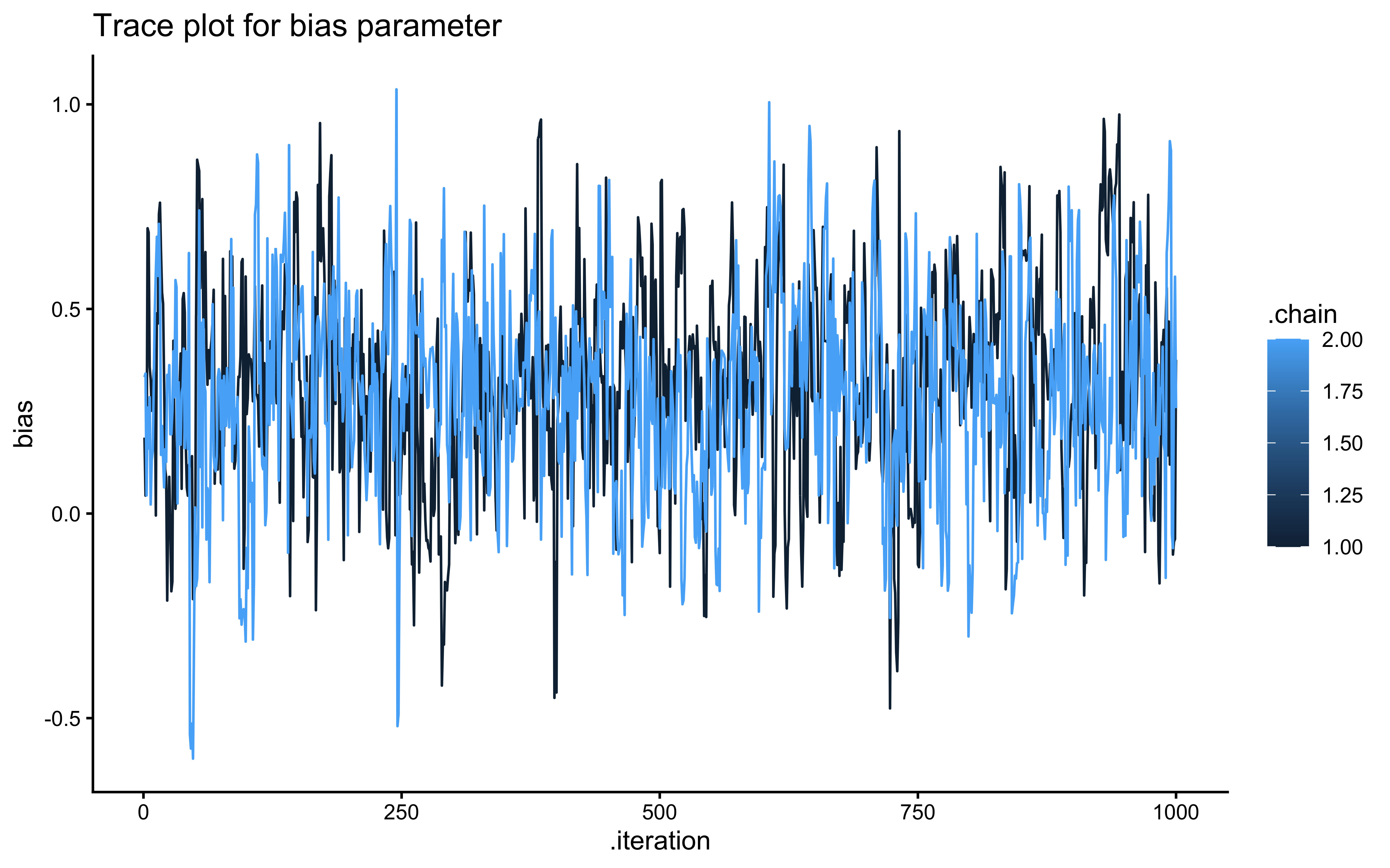
# Trace plot for bias
ggplot(draws_df_memory, aes(.iteration, bias, group = .chain, color = .chain)) +
  geom_line() +
  labs(title = "Trace plot for bias parameter") +
  theme_classic()
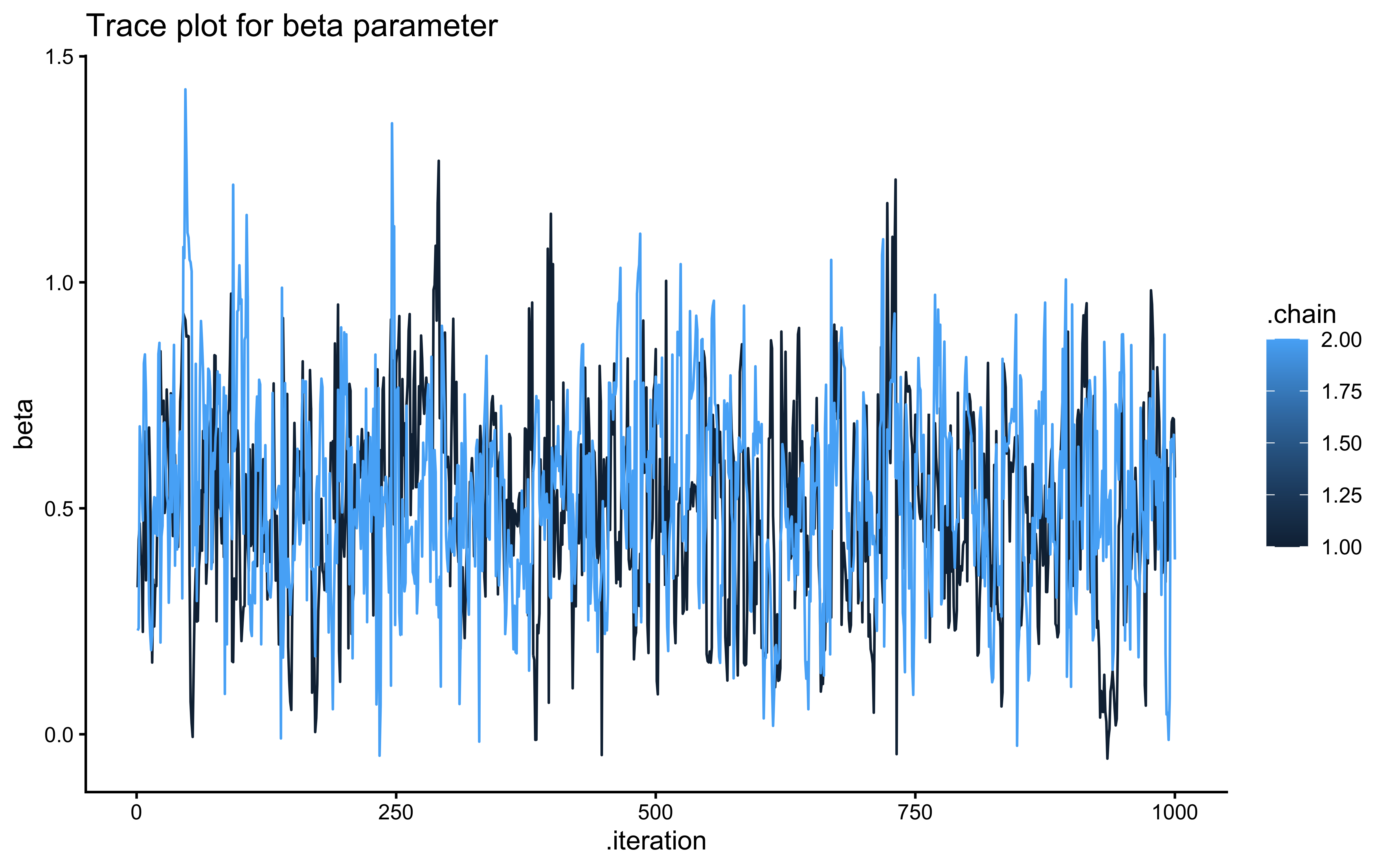
# Trace plot for beta
ggplot(draws_df_memory, aes(.iteration, beta, group = .chain, color = .chain)) +
  geom_line() +
  labs(title = "Trace plot for beta parameter") +
  theme_classic()
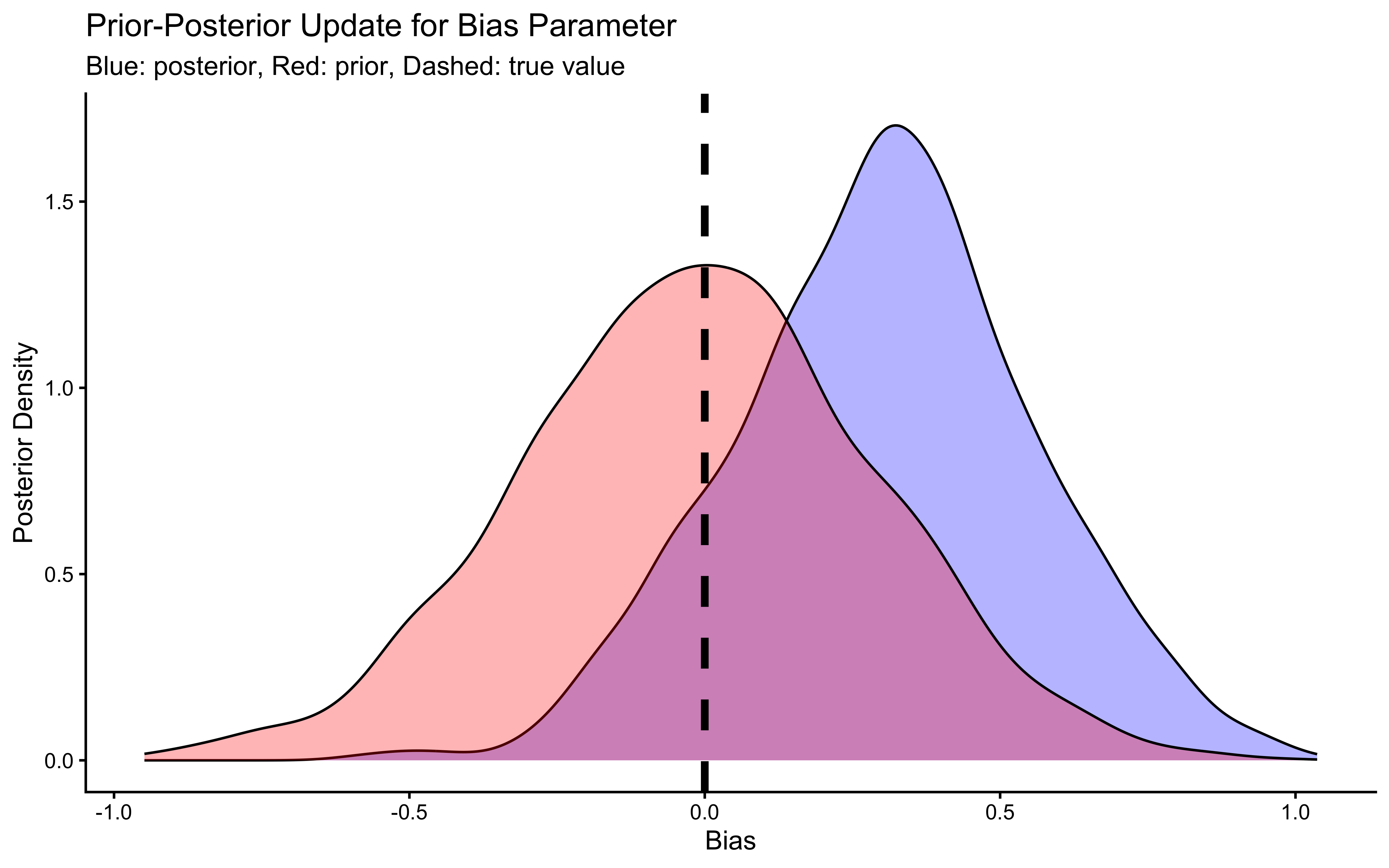
# Now let's plot the density for bias (prior and posterior)
ggplot(draws_df_memory) +
  geom_density(aes(bias), fill = "blue", alpha = 0.3) +
  geom_density(aes(bias_prior), fill = "red", alpha = 0.3) +
  geom_vline(xintercept = 0, linetype = "dashed", color = "black", size = 1.5) +
  labs(title = "Prior-Posterior Update for Bias Parameter",
       subtitle = "Blue: posterior, Red: prior, Dashed: true value") +
  xlab("Bias") +
  ylab("Posterior Density") +
  theme_classic()
# Now let's plot the density for beta (prior and posterior)
ggplot(draws_df_memory) +
geom_density(aes(beta), fill = "blue", alpha = 0.3) +
geom_density(aes(beta_prior), fill = "red", alpha = 0.3) +
geom_vline(xintercept = 1, linetype = "dashed", color = "black", size = 1.5) +
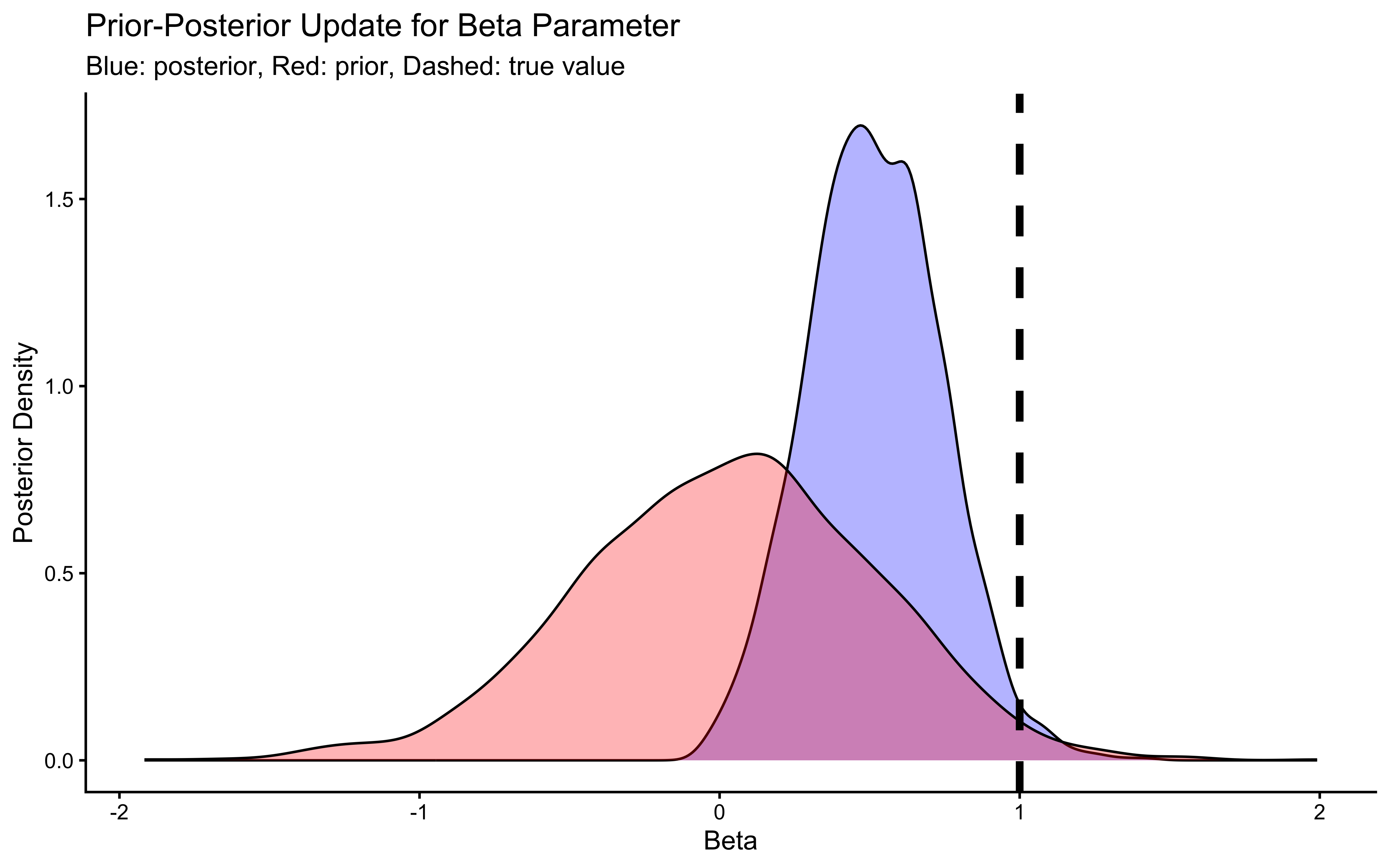
labs(title = "Prior-Posterior Update for Beta Parameter",
subtitle = "Blue: posterior, Red: prior, Dashed: true value") +
xlab("Beta") +
ylab("Posterior Density") +
theme_classic()
# Print summary
samples_memory$summary()
```
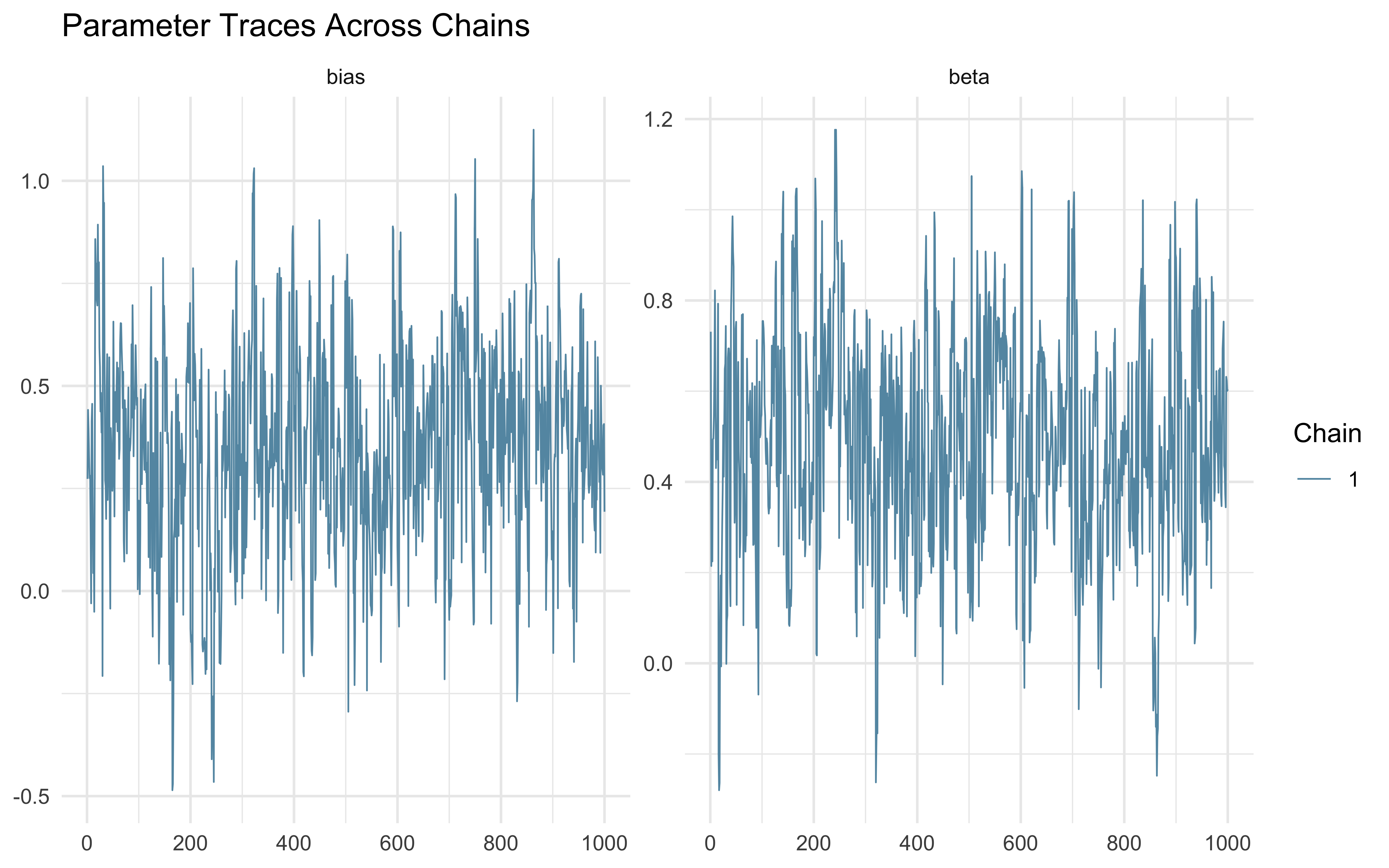
The trace plots should show the same "hairy caterpillar" pattern as before — well-mixed chains with no systematic drift. The prior-posterior update plots tell the story: the posterior for `bias` should be narrow and centred near 0 (log-odds of 0.5 = unbiased), and the posterior for `beta` should be centred near 1 (the true generating value). The data have meaningfully updated both parameters away from their priors. Formal quality checks — prior predictive checks, systematic parameter recovery, and SBC — come in Ch. 6.
### Memory Model 2: Internal State Variable
Instead of feeding memory as external data, we can model it as an internal state that updates within the model.
For this specific model — where memory is simply a running average of the opponent's choices — the update rule depends only on the observed data (`other`), not on any parameter being estimated. We should therefore calculate it in Stan's `transformed data` block.
::: {.callout-tip title="Stan Efficiency Rule 1 — Block Placement: Run it Once, Not Thousands of Times"}
Every Stan model has blocks that execute at very different frequencies. Choosing the **right block** is the most impactful single optimization:
| Block | Executes | Use for |
|---|---|---|
| `transformed data` | **Once**, before sampling | Any quantity derived **only from data** — precomputed distances, normalized inputs, log-transforms of fixed constants |
| `transformed parameters` | **Every leapfrog step** | Deterministic functions of parameters whose gradients must flow backward — recursive states, reparameterizations, predicted values used in the likelihood |
| `model` (local `{}` block) | Every leapfrog step, **not saved** | Scratch variables for accumulating `target +=`; no overhead from the saved-draw tape |
| `generated quantities` | **Once per saved draw** (post-warmup only) | PPCs, log-likelihoods, prior samples — expensive quantities you only need in the final posterior |
**Concrete cost of misplacement.** A typical fit runs 4 chains × 1000 warmup × ~6 leapfrog steps per draw = ~24 000 leapfrog evaluations. Any computation in `transformed parameters` runs ~24 000 times. The same computation in `transformed data` runs exactly once. For a model with 500 trials, precomputing 500 memory values in `transformed data` rather than `transformed parameters` saves ~12 million floating-point operations per fit.
**The decision tree:**
1. Does this depend **only on data** (not on any parameter)?
→ `transformed data`
2. Does this depend on **parameters** and does the likelihood or another parameter need it?
→ `transformed parameters`
3. Is this needed **only after sampling** (PPC draws, LOO log-likelihoods)?
→ `generated quantities`, gated by `run_diagnostics` (introduced properly in Ch. 5)
4. Is this just a temporary accumulator inside a loop?
→ Local variable inside `{}` in `model` or `transformed parameters`
In the memory model below, `memory` depends only on `other` (data) → `transformed data`. In the forgetting model that follows, `memory` depends on the free parameter `forgetting` → local variable inside `model`.
**Corollary — pre-compute in R when possible.** If a quantity depends only on data and will
never change between fits, computing it in R and passing it as a data field is even faster than
`transformed data`: Stan never sees the raw computation at all. For example, the multilevel
memory model in Chapter 6 pre-computes the running opponent rate in R and passes `opp_rate_prev`
as a vector, rather than recomputing it inside Stan on every chain.
:::
::: {.callout-tip title="Stan Efficiency — Vectorize the Likelihood Call"}
Stan evaluates each `~` or `target +=` statement as a separate autodiff node.
Replacing a trial-level loop with a **vectorized distribution call** collapses $N$ nodes
into one, reducing autodiff graph size and improving cache locality.
```stan
// Slower: N separate nodes in the autodiff graph
for (i in 1:N)
  target += bernoulli_logit_lpmf(h[i] | theta_logit);

// Faster: one vectorized call — h and theta_logit are both length-N vectors
target += bernoulli_logit_lpmf(h | theta_logit);
```
The vectorized form works whenever `theta_logit` is either a **scalar** (broadcasts to all
trials) or a **vector of the same length as `h`**. In the multilevel model of Chapter 6,
`target += bernoulli_logit_lpmf(y | theta_logit[subj_id])` vectorizes the full N_total
trial loop by scatter-indexing the per-subject parameters.
**Caveat:** vectorization is not available for mixture likelihoods (`log_mix`) because each
observation requires its own separate `log_mix` call. The loop is unavoidable there (Ch. 8).
:::
```{r ch05_internal memory stan model}
## Create the data — run_diagnostics = 1 for the single validation fit
data <- list(
  n = 120,
  h = d1$Self,
  other = d1$Other,
  run_diagnostics = 1L
)

stan_model <- "
// Memory-based choice model with prior and posterior predictions.
// memory[] is data-derived and lives in transformed data (computed once).
// run_diagnostics gates expensive generated quantities for SBC speed.

data {
 int<lower=1> n;
 array[n] int h;
 array[n] int other;
 int<lower=0, upper=1> run_diagnostics; // 1 = compute PPC + log_lik; 0 = skip (use for SBC)
}

transformed data {
  // memory depends only on other[] (data), so it runs ONCE here.
  // Moving this to transformed parameters would recompute it ~24 000 times per fit.
  vector[n] memory;
  memory[1] = 0.5;
  for (trial in 1:(n-1)) {
     memory[trial + 1] = memory[trial] + ((other[trial] - memory[trial]) / (trial + 1));
     if (memory[trial + 1] < 0.01) memory[trial + 1] = 0.01;
     if (memory[trial + 1] > 0.99) memory[trial + 1] = 0.99;
  }
}

parameters {
  real bias;
  real beta;
}

model {
  target += normal_lpdf(bias | 0, .3);
  target += normal_lpdf(beta | 0, .5);
  // Vectorized likelihood — no loop needed because memory is precomputed.
  target += bernoulli_logit_lpmf(h | bias + beta * logit(memory));
}

generated quantities {
  // Prior samples are always generated (cheap).
  real bias_prior = normal_rng(0, 0.3);
  real beta_prior = normal_rng(0, 0.5);
  // Expensive diagnostics are gated — set run_diagnostics = 0 during SBC.
  vector[n] log_lik;
  array[n] int y_rep;
  if (run_diagnostics) {
    for (trial in 1:n) {
      log_lik[trial] = bernoulli_logit_lpmf(h[trial] | bias + beta * logit(memory[trial]));
      y_rep[trial]   = bernoulli_logit_rng(bias + beta * logit(memory[trial]));
    }
  }
}
"

write_stan_file(
  stan_model,
  dir = "stan/",
  basename = "ch06_InternalMemory.stan")
## Specify where the model is
file <- here("stan", "ch06_InternalMemory.stan")

# File path for saved model
model_file <- here("simmodels", "ch06_InternalMemory.rds")

# Check if we need to rerun the simulation
if (regenerate_simulations || !file.exists(model_file)) {
  # Compile the model
  mod <- cmdstan_model(file,
                       cpp_options = list(stan_threads = FALSE),
                       stanc_options = list("O1"))

  # The following command calls Stan with specific options.
  samples_memory_internal <- mod$sample(
    data = data,
    seed = 123,
    chains = 1,
    parallel_chains = 2,
    threads_per_chain = 1,
    iter_warmup = 1000,
    iter_sampling = 1000,
    refresh = 0,
    max_treedepth = 20,
    adapt_delta = 0.99,
  )

  # Save the fitted model
  samples_memory_internal$save_object(file = model_file)
  cat("Generated new model fit and saved to", model_file, "\n")
} else {
  # Load existing results
  samples_memory_internal <- readRDS(model_file)
  cat("Loaded existing model fit from", model_file, "\n")
}
draws_df <- as_draws_df(samples_memory_internal$draws())

# 1. Check chain convergence
# Plot traces for main parameters
mcmc_trace(draws_df, pars = c("bias", "beta")) +
  theme_minimal() +
  ggtitle("Parameter Traces Across Chains")
# Plot rank histograms to check mixing
mcmc_rank_hist(draws_df, pars = c("bias", "beta"))
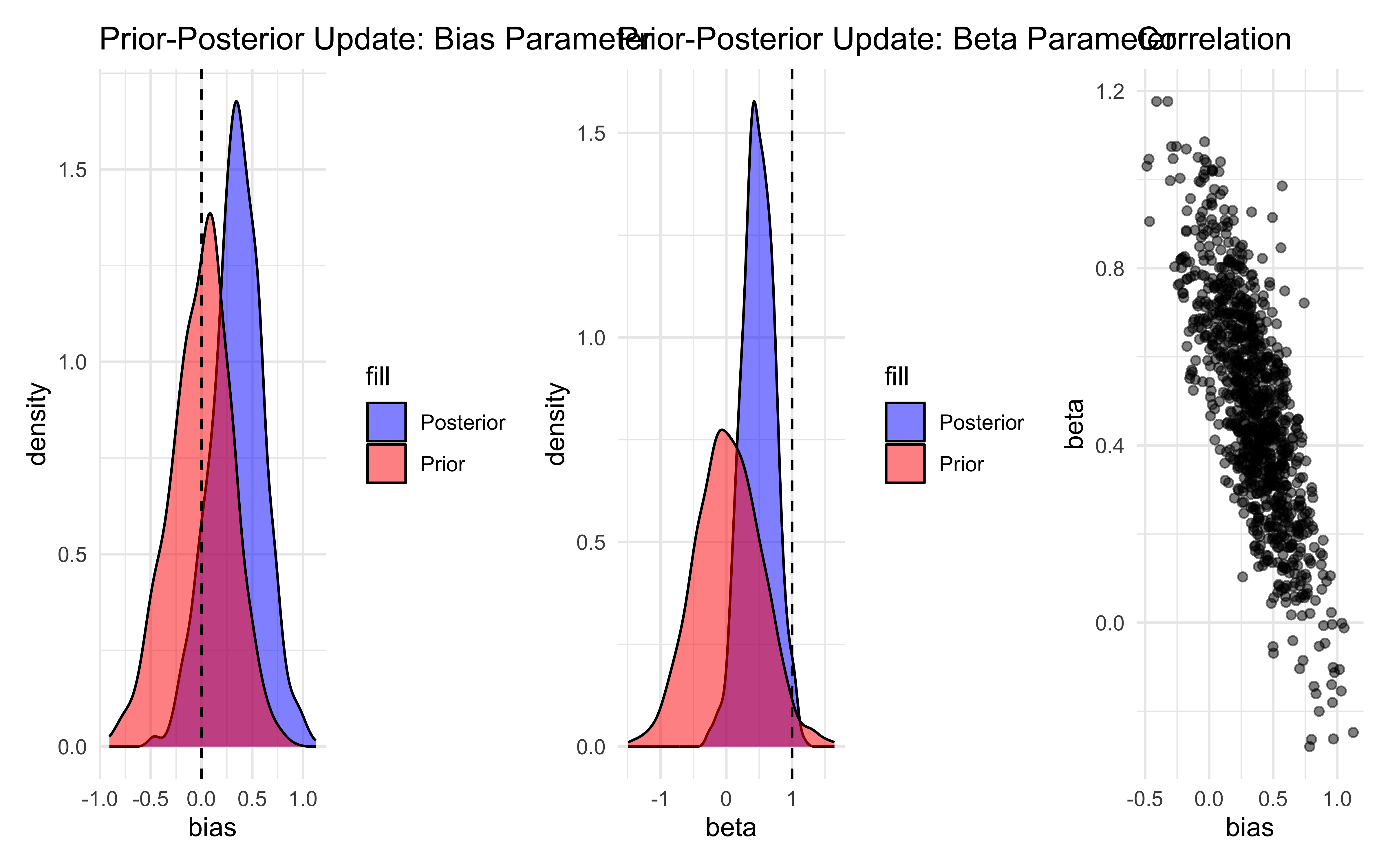
# 2. Prior-Posterior Update Check
p1 <- ggplot() +
  geom_density(data = draws_df, aes(bias, fill = "Posterior"), alpha = 0.5) +
  geom_density(data = draws_df, aes(bias_prior, fill = "Prior"), alpha = 0.5) +
  geom_vline(xintercept = 0, linetype = "dashed") +
  scale_fill_manual(values = c("Prior" = "red", "Posterior" = "blue")) +
  theme_minimal() +
  ggtitle("Prior-Posterior Update: Bias Parameter")

p2 <- ggplot() +
  geom_density(data = draws_df, aes(beta, fill = "Posterior"), alpha = 0.5) +
  geom_density(data = draws_df, aes(beta_prior, fill = "Prior"), alpha = 0.5) +
  geom_vline(xintercept = 1, linetype = "dashed") +
  scale_fill_manual(values = c("Prior" = "red", "Posterior" = "blue")) +
  theme_minimal() +
  ggtitle("Prior-Posterior Update: Beta Parameter")

p3 <- ggplot() +
  geom_point(data = draws_df, aes(bias, beta), alpha = 0.5) +
  theme_minimal() +
  ggtitle("Correlation")

p1 + p2 + p3
```
Now that we know how to model memory as an internal state, we can play with making the update discount the past, setting a parameter that indicates after how many trials memory is lost, etc.
### Memory Model 3: Exponential Forgetting (similar to RL)
A more cognitively plausible memory model incorporates forgetting, where recent events have more influence than distant ones. This can be implemented by adding a `forgetting` parameter (often called a learning rate, α, in RL) that controls the weight of the most recent outcome versus the previous memory state.
```{r ch05_internal memory with forgetting stan model}
stan_model <- "
// Memory model with exponential forgetting (learning-rate style).
// memory[] depends on the free parameter 'forgetting', so it cannot go in
// transformed data. It lives as a local vector inside the model block —
// computed at every leapfrog step but never saved to the posterior draws.

data {
  int<lower=1> n;
  array[n] int h;
  array[n] int other;
  int<lower=0, upper=1> run_diagnostics;
}

parameters {
  real bias;
  real beta;
  real<lower=0, upper=1> forgetting;
}

model {
  target += beta_lpdf(forgetting | 1, 1);
  target += normal_lpdf(bias | 0, .3);
  target += normal_lpdf(beta | 0, .5);

  // memory is a LOCAL variable — declared inside model, so it lives on the
  // stack and is discarded after each leapfrog step without touching the saved-
  // draw tape. This is the right pattern when memory depends on a parameter.
  vector[n] memory;
  for (trial in 1:n) {
    if (trial == 1) memory[trial] = 0.5;
    target += bernoulli_logit_lpmf(h[trial] | bias + beta * logit(memory[trial]));
    if (trial < n) {
      memory[trial + 1] = (1 - forgetting) * memory[trial] + forgetting * other[trial];
      if (memory[trial + 1] <= 0) memory[trial + 1] = 0.01;
      if (memory[trial + 1] >= 1) memory[trial + 1] = 0.99;
    }
  }
}

generated quantities {
  real bias_prior      = normal_rng(0, 0.3);
  real beta_prior      = normal_rng(0, 0.5);
  real forgetting_prior = beta_rng(1, 1);
  vector[n] log_lik;
  array[n] int y_rep;
  if (run_diagnostics) {
    // Recompute memory for the saved draw — runs once per posterior sample.
    vector[n] memory_gq;
    for (trial in 1:n) {
      if (trial == 1) memory_gq[trial] = 0.5;
      real lin = bias + beta * logit(memory_gq[trial]);
      log_lik[trial] = bernoulli_logit_lpmf(h[trial] | lin);
      y_rep[trial]   = bernoulli_logit_rng(lin);
      if (trial < n) {
        memory_gq[trial + 1] = (1 - forgetting) * memory_gq[trial] + forgetting * other[trial];
        if (memory_gq[trial + 1] <= 0) memory_gq[trial + 1] = 0.01;
        if (memory_gq[trial + 1] >= 1) memory_gq[trial + 1] = 0.99;
      }
    }
  }
}
"
write_stan_file(
  stan_model,
  dir = "stan/",
  basename = "ch06_InternalMemory2.stan")
## Specify where the model is
file <- here("stan","ch06_InternalMemory2.stan")

# File path for saved model
model_file <- here("simmodels","ch06_InternalMemory2.rds")

# Check if we need to rerun the simulation
if (regenerate_simulations || !file.exists(model_file)) {
  # Compile the model
  mod <- cmdstan_model(file,
                       cpp_options = list(stan_threads = FALSE),
                       stanc_options = list("O1"))

  data_forgetting <- modifyList(data, list(run_diagnostics = 1L))
  # The following command calls Stan with specific options.
  samples_memory_forgetting <- mod$sample(
    data = data_forgetting,
    seed = 123,
    chains = 4,
    parallel_chains = 4,
    iter_warmup = 1000,
    iter_sampling = 1000,
    refresh = 0,
    adapt_delta = 0.95
  )

  # Save the fitted model
  samples_memory_forgetting$save_object(file = model_file)
  cat("Generated new model fit and saved to", model_file, "\n")
} else {
  # Load existing results
  samples_memory_forgetting <- readRDS(model_file)
  cat("Loaded existing model fit from", model_file, "\n")
}
samples_memory_forgetting$summary()
```
The memory model we've implemented can be seen as part of a broader family of models that track and update beliefs based on incoming evidence. Let's explore how it relates to some key frameworks.
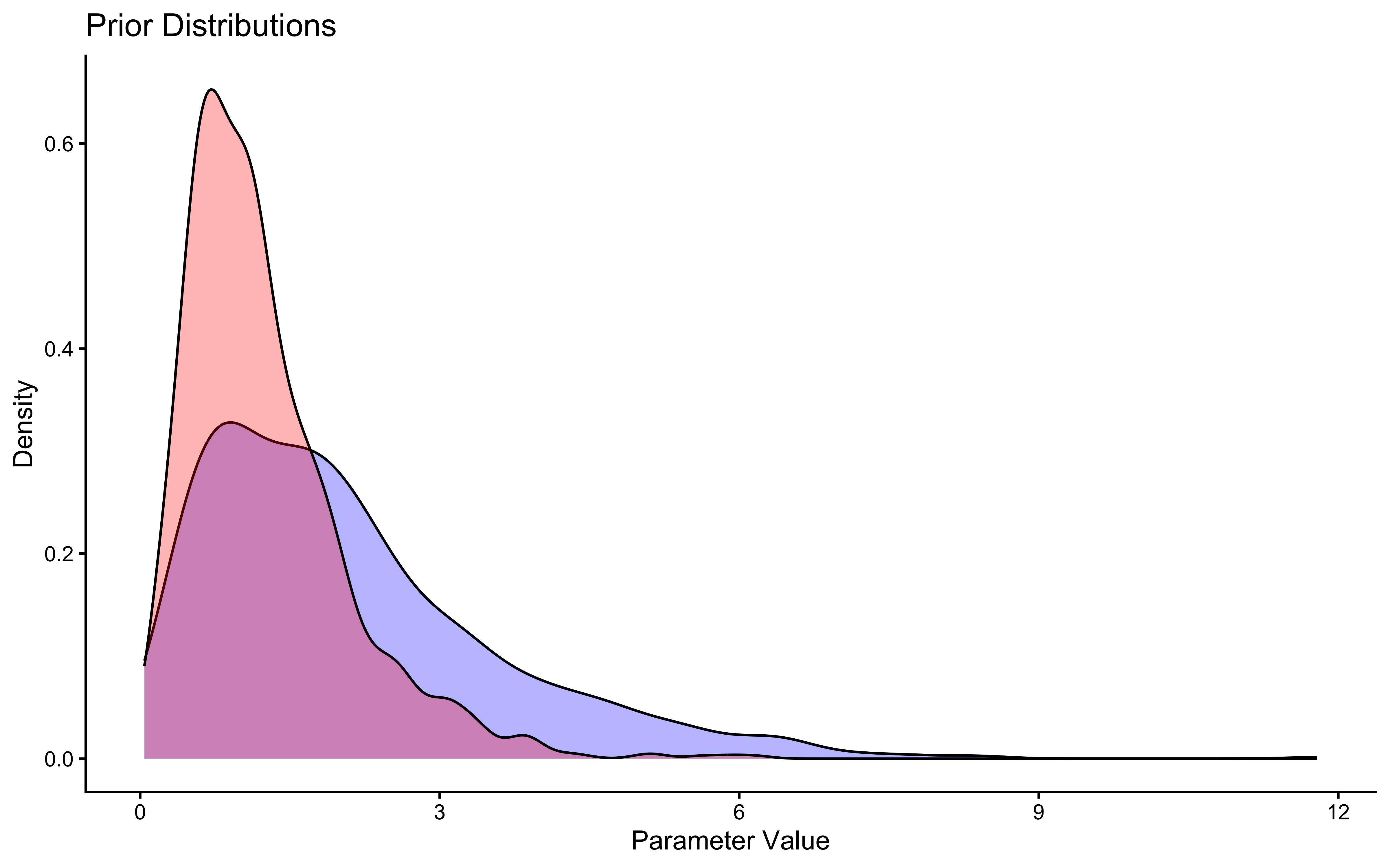
## Memory Model 4: Bayesian Agent (Optimal Updating)
A fully Bayesian agent wouldn't just track the rate but maintain a full probability distribution (a Beta distribution) over the likely bias of the opponent, updating it optimally according to Bayes' rule after each observation.
```{r ch05_bayesian memory stan model}
stan_model <- "
data {
  int<lower=1> n;  // number of trials
  array[n] int h;  // agent's choices (0 or 1)
  array[n] int other;  // other player's choices (0 or 1)
}

parameters {
  real<lower=0> alpha_prior;  // Prior alpha parameter
  real<lower=0> beta_prior;   // Prior beta parameter
}

transformed parameters {
  vector[n] alpha;  // Alpha parameter at each trial
  vector[n] beta;   // Beta parameter at each trial
  vector[n] rate;   // Expected rate at each trial

  // Initialize with prior
  alpha[1] = alpha_prior;
  beta[1] = beta_prior;
  rate[1] = alpha[1] / (alpha[1] + beta[1]);

  // Sequential updating of Beta distribution
  for(t in 2:n) {
    // Update Beta parameters based on previous observation
    alpha[t] = alpha[t-1] + other[t-1];
    beta[t] = beta[t-1] + (1 - other[t-1]);

    // Calculate expected rate
    rate[t] = alpha[t] / (alpha[t] + beta[t]);
  }
}

model {
  // Priors on hyperparameters
  target += gamma_lpdf(alpha_prior | 2, 1);
  target += gamma_lpdf(beta_prior | 2, 1);

  // Agent's choices follow current rate estimates
  for(t in 1:n) {
    target += bernoulli_lpmf(h[t] | rate[t]);
  }
}

generated quantities {
  // We strictly reserve posterior predictive checks for Chapter 6.
  // Here, we just calculate the initial expected rate for reference.
  real initial_rate = alpha_prior / (alpha_prior + beta_prior);
}
"
write_stan_file(
  stan_model,
  dir = "stan/",
  basename = "ch06_BayesianMemory.stan")
## Specify where the model is
file <- here("stan","ch06_BayesianMemory.stan")

# File path for saved model
model_file <- here("simmodels","ch06_BayesianMemory.rds")

# Check if we need to rerun the simulation
if (regenerate_simulations || !file.exists(model_file)) {
  # Compile the model
  mod <- cmdstan_model(file)

  # The following command calls Stan with specific options.
  samples_memory_bayes <- mod$sample(
    data = data,
    seed = 123,
    chains = 1,
    parallel_chains = 2,
    threads_per_chain = 1,
    iter_warmup = 1000,
    iter_sampling = 1000,
    refresh = 0,
    max_treedepth = 20,
    adapt_delta = 0.99,
  )

  # Save the fitted model
  samples_memory_bayes$save_object(file = model_file)
  cat("Generated new model fit and saved to", model_file, "\n")
} else {
  # Load existing results
  samples_memory_bayes <- readRDS(model_file)
  cat("Loaded existing model fit from", model_file, "\n")
}
samples_memory_bayes$summary()
# Extract draws
draws_df <- as_draws_df(samples_memory_bayes$draws())

# First let's look at the priors
ggplot(draws_df) +
  geom_density(aes(alpha_prior), fill = "blue", alpha = 0.3) +
  geom_density(aes(beta_prior), fill = "red", alpha = 0.3) +
  theme_classic() +
  labs(title = "Prior Distributions",
       x = "Parameter Value",
       y = "Density")
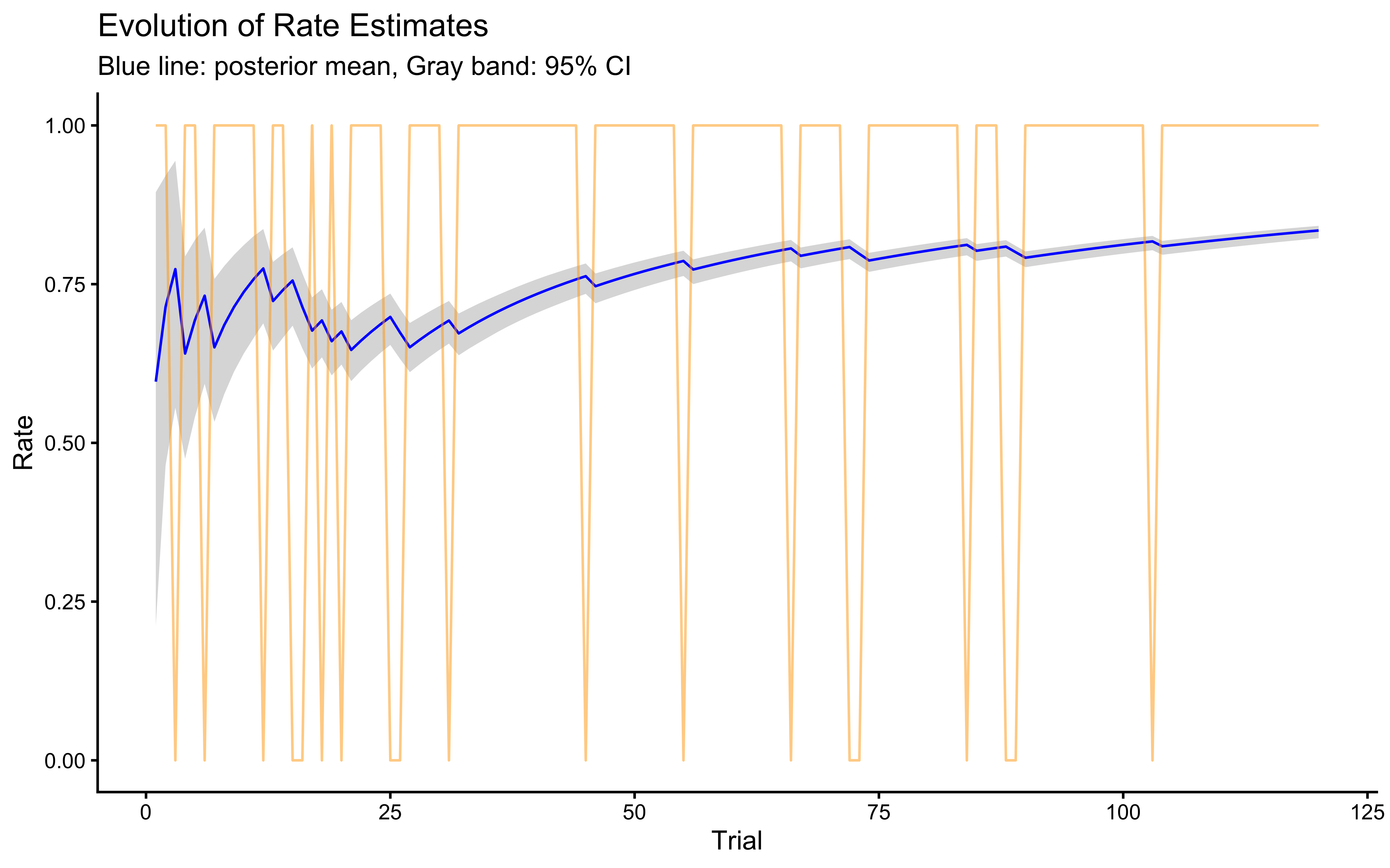
# Now let's look at how the rate evolves over trials
# First melt the rate values across trials into long format
rate_df <- draws_df %>%
  dplyr::select(starts_with("rate[")) %>%
  pivot_longer(everything(),
               names_to = "trial",
               values_to = "rate",
               names_pattern = "rate\\[(\\d+)\\]") %>%
  mutate(trial = as.numeric(trial))

# Calculate summary statistics for each trial
rate_summary <- rate_df %>%
  group_by(trial) %>%
  summarise(
    mean_rate = mean(rate),
    lower = quantile(rate, 0.025),
    upper = quantile(rate, 0.975)
  )


plot_data <- tibble(trial = seq(120), choices = data$other)

# Plot the evolution of rate estimates
ggplot(rate_summary, aes(x = trial)) +
  geom_ribbon(aes(ymin = lower, ymax = upper), alpha = 0.2) +
  geom_line(aes(y = mean_rate), color = "blue") +
  # Add true data points
  geom_line(data = plot_data,
             aes(x = trial, y = choices), color = "orange", alpha = 0.5) +
  theme_classic() +
  labs(title = "Evolution of Rate Estimates",
       x = "Trial",
       y = "Rate",
       subtitle = "Blue line: posterior mean, Gray band: 95% CI") +
  ylim(0, 1)
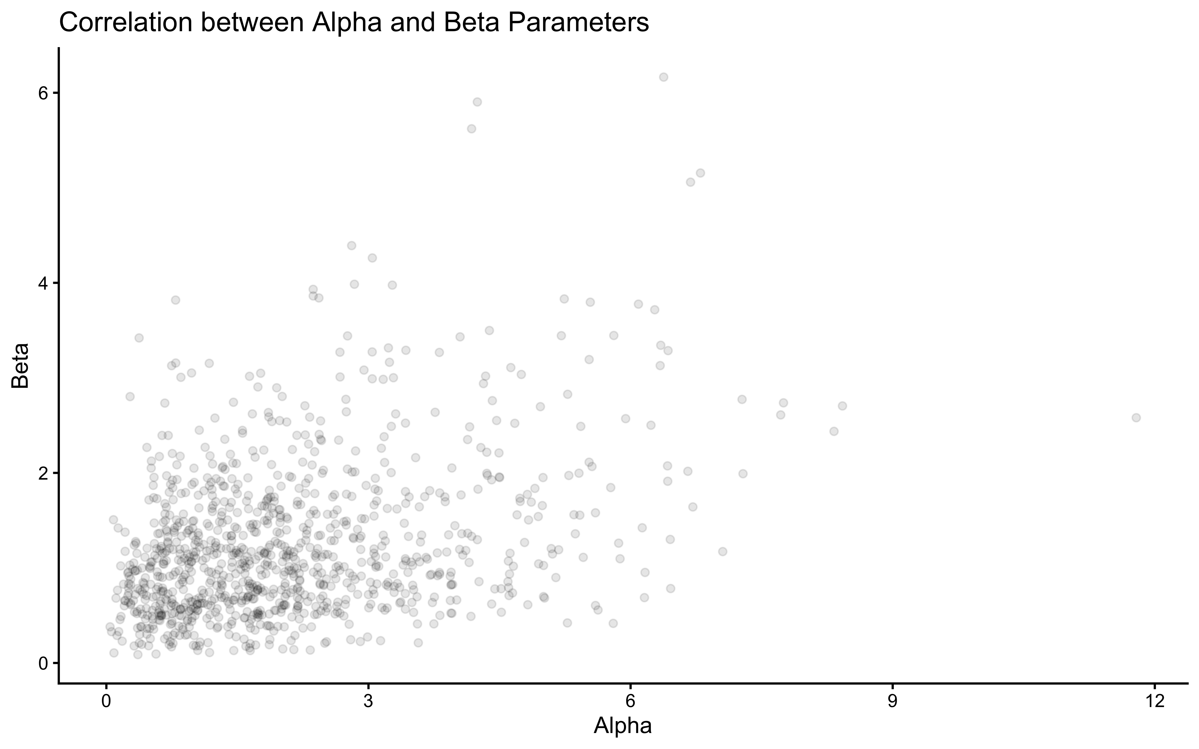
# Let's also look at the correlation between alpha and beta parameters
ggplot(draws_df) +
  geom_point(aes(alpha_prior, beta_prior), alpha = 0.1) +
  theme_classic() +
  labs(title = "Correlation between Alpha and Beta Parameters",
       x = "Alpha",
       y = "Beta")
```
## Relationship to Rescorla-Wagner
The Rescorla-Wagner model of learning—which drives the Reinforcement Learning agents we will build in in a later chapter follows the form:
$$V_{t+1} = V_{t} + \alpha (R_{t} - V_{t})$$
where:
* $V_{t}$ is the current Value estimate (in our code: memory[t]).
* $\alpha$ is the Learning Rate (in our code: forgetting).
* $R_{t}$ is the Reward or Outcome (in our code: other[t]).
* $(R_{t} - V_{t})$ is the Prediction Error.
Our memory model with a forgetting parameter follows a very similar structure:$$\text{memory}_{t+1} = (1 - \text{forgetting}) \times \text{memory}_{t} + \text{forgetting} \times \text{outcome}_{t}$$If we expand this, we can see it is mathematically identical to the Rescorla-Wagner update rule:$$\begin{aligned}
\text{memory}_{t+1} &= \text{memory}_{t} - \text{forgetting} \times \text{memory}_{t} + \text{forgetting} \times \text{outcome}_{t} \\
\text{memory}_{t+1} &= \text{memory}_{t} + \text{forgetting} \times (\text{outcome}_{t} - \text{memory}_{t})
\end{aligned}$$
This reveals that our "exponential forgetting" memory model is actually a standard Reinforcement Learning agent with a big fake moustache. The forgetting parameter dictates how quickly the agent updates their beliefs (value estimate) based on new prediction errors.
### Connection to Kalman Filters
Our memory model updates beliefs about the probability of right-hand choices using a weighted average of past observations. This is conceptually similar to how a Kalman filter works, though simpler:
* Kalman filters maintain both an estimate and uncertainty about that estimate
* They optimally weight new evidence based on relative uncertainty
* Our forgetting model uses a fixed weighting scheme (1/trial or the forgetting parameter)
* The Bayesian Agent (`ch06_BayesianMemory.stan`) captures uncertainty via the Beta distribution, similar in spirit but simpler than a Kalman filter.
### Connection to Hierarchical Gaussian Filter (HGF)
The HGF extends these ideas by:
* Tracking beliefs at multiple levels
* Allowing learning rates to vary over time
* Explicitly modeling environmental volatility
Our model could be seen as the simplest case of an HGF where:
* We only track one level (probability of right-hand choice)
* Have a fixed learning rate (forgetting parameter)
* Don't explicitly model environmental volatility
### Implications for Model Development
Understanding these relationships helps us think about how models relate to each other and to extend our model:
* We could add uncertainty estimates to get Kalman-like behavior
* We could make the forgetting parameter dynamic to capture changing learning rates
* We could add multiple levels to track both immediate probabilities and longer-term trends
Each extension would make the model more flexible but also more complex to fit to data. The choice depends on our specific research questions and available data.
## Conclusion: Estimating Parameters and Exploring Memory
This chapter marked a crucial transition from simulating models with known parameters to the core task of **parameter estimation**: inferring plausible parameter values from observed data using Bayesian inference and Stan.
We learned how to:
* **Specify Bayesian models** in Stan, defining data, parameters, priors, and data models.
* **Fit models** using `cmdstanr` to obtain posterior distributions for parameters like choice bias (`theta`).
* **Utilize transformations** like log-odds for computational benefits and flexible prior specification.
* **Validate our fitting procedure** through **parameter recovery**, ensuring our models can retrieve known values from simulated data.
* **Implement different cognitive models** for history-dependent choice, exploring various ways to represent **memory**: as an external predictor, an internal updating state, incorporating exponential forgetting (linking to Reinforcement Learning principles), and even as a fully Bayesian belief update.
* **Recognize connections** between these models and broader frameworks like Kalman filters and HGF.
By fitting these models, we moved beyond simply describing behavior (like the cumulative rates in Chapter 3) to quantifying underlying latent parameters (like `bias`, `beta`, `forgetting`).
However, a single fit to a single simulated dataset is only a preliminary
sanity check — the equivalent of flipping a coin once to check if it's fair.
It does not tell us whether the model behaves well across a wide range of
parameter values, whether our credible intervals are correctly calibrated, or
whether the fitted model can actually reproduce the patterns in the data.
**Coming up in Chapter 6:** We take the Stan models built in this chapter and
subject them to a four-phase validation battery before they are allowed near
real human data:
1. **Prior Predictive Check** — do the priors allow only cognitively plausible behavior?
2. **Parameter Recovery** — does the model find the right answer across many simulated datasets and noise levels?
3. **Simulation-Based Calibration Checks (SBC)** — are our posterior intervals actually calibrated (does a 95% CI contain the truth 95% of the time)?
4. **Posterior Predictive Check** — does the fitted model reproduce key patterns in the observed data?
Only after passing all four tests does a model earn the right to touch real
empirical data.