---
title: "Rule-Based Categorization Models (v2 — BayesFlow workflow)"
format:
html:
code-fold: true
code-tools: true
---
# Categorization models: Rules {#sec-rules}
::: {.callout-important title="What changed in v2"}
This is a revision of Chapter 15 in which the Neural Posterior Estimation
pipeline has been re-implemented on top of the **BayesFlow 2.x amortized
Bayesian workflow** instead of `sbi` + `reticulate`.
Concretely:
* The neural architecture is now a `TimeSeriesTransformer` summary network
(the trial sequence is ordered and path-dependent — it is structured data,
not a flat covariate vector) followed by a `FlowMatching` inference network.
* Routing is handled by an explicit `bf.Adapter()` chain, and training uses
`workflow.fit_offline` with a held-out validation set.
* In-silico diagnostics are produced by `workflow.compute_default_diagnostics`
and `workflow.plot_default_diagnostics`; hand-rolled SBC / coverage code
has been removed.
* The prior on the working-memory bound has been narrowed from
`Uniform(log 20, log 300)` to `Uniform(log 1, log 100)`, addressing the
cognitive-plausibility concern raised in the v1 placeholder box.
* Heavy compute (simulation + training) is no longer executed inline via
`reticulate`. It is delegated to a standalone Python script,
`scripts/ucloud_npe/amortized_particle_filter.py`, which is intended to be
run on uCloud (or any GPU/CPU node with JAX). The chapter loads the
resulting artifacts (`metrics.csv`, posterior samples, `history.json`) for
presentation.
All diagnostic plots are generated as inline ggplot2 panels reading CSV files exported by the standalone Python script, consistent with the visual conventions of the rest of the book.
:::
```{r ch15_setup, include=FALSE}
knitr::opts_chunk$set(
echo = TRUE,
message = FALSE,
warning = FALSE,
fig.width = 8,
fig.height = 5,
fig.align = "center",
out.width = "80%",
dpi = 300
)
# Set to TRUE to rerun simulations and Stan fits.
# FALSE loads pre-computed results from 'simdata/'.
regenerate_simulations <- FALSE
# Set to TRUE to run the long-running validation chunks
# (rule-set sensitivity, real SBC for the Stan proxy, NPE pipeline,
# coverage validation, NPE-vs-Stan comparison).
run_intensive_checks <- FALSE
pacman::p_load(
tidyverse, # data manipulation and visualization
patchwork, # combining plots
cmdstanr, # Stan interface
posterior, # tidy posterior arrays
tidybayes, # tidy extraction of draws
bayesplot, # MCMC diagnostic plots
loo, # LOO-CV and PSIS
SBC, # Simulation-Based Calibration Checks
priorsense, # prior sensitivity
future, # parallel processing
furrr, # parallel functional programming
matrixStats, # logSumExp for PSIS calculations
reticulate, # Python interop for sbi / BayesFlow
slider, # rolling window summaries
ggrepel, # non-overlapping text labels
here
)
theme_set(theme_classic())
# ── NPE artifacts produced off-host ──────────────────────────────────────────
# v2: training and simulation run in scripts/ucloud_npe/amortized_particle_filter.py.
# The script writes per-scenario artifacts under
# simdata/ch15_v2_bayesflow/<scenario>/
# where <scenario> is one of: static, contingent_shift, drift.
# The chapter's "main" NPE chunks read from the static run; the scenario
# subsections read from contingent_shift / drift.
python_available <- FALSE
npe_artifacts_root <- here("simdata", "ch15_v2_bayesflow")
NPE_SCENARIOS <- c("static", "contingent_shift", "drift")
npe_scenario_dir <- function(s) file.path(npe_artifacts_root, s)
npe_scenario_ready <- function(s) {
d <- npe_scenario_dir(s)
dir.exists(d) && file.exists(file.path(d, "metrics.csv"))
}
# Default scenario for the main NPE block (Step 1–4 in the chapter):
npe_artifacts_dir <- npe_scenario_dir("static")
npe_artifacts_available <- npe_scenario_ready("static")
# ── Prior hyperparameter for logit(error_prob) ────────────────────────────────
# Normal(0, 1.5) is approximately uniform on the probability scale.
# Prior median ε ≈ 0.50; 95% mass on (0.05, 0.95).
# This is deliberately wider than the Normal(-2, 1) used in earlier drafts,
# which concentrated mass below ε = 0.27 and cut off the posterior for
# near-chance subjects. priorsense::powerscale_sensitivity() should be
# checked; if ψ > 0.1 for any quantity, the prior matters and this choice
# must be defended.
LOGIT_ERROR_PRIOR_MEAN <- 0.0
LOGIT_ERROR_PRIOR_SD <- 1.5
# ── Prior hyperparameter for logit(mutation_prob) ─────────────────────────────
# logit(μ) ~ Normal(-3, 1.5): prior median μ ≈ 0.047, 95% mass on (0.003, 0.37).
# This reflects the cognitive prior that most learners mutate rarely on any
# given trial — μ = 0 (static filter) is the default baseline. The SD is wide
# enough to accommodate highly adaptive learners (μ ≈ 0.2–0.3) while keeping
# most prior mass below 0.15. On static data we expect the posterior to be
# largely prior-like; on non-stationary data it should sharpen.
LOGIT_MU_PRIOR_MEAN <- -3.0
LOGIT_MU_PRIOR_SD <- 1.5
# ── Development-mode switch ───────────────────────────────────────────────────
# Set DEV_MODE <- TRUE when iterating on the chapter on a laptop (M1 or similar).
# This halves particle count and training simulations, cutting wall time by ~50–60%.
# Set FALSE for the final publication run so all structural choices match the text.
DEV_MODE <- FALSE
# ── Structural commitments for the particle filter (Model A) ─────────────────
# These are NOT inferred from data — they are cognitive choices the modeller
# makes. Sensitivity to each is exercised in dedicated subsections.
# Publication value: 100. DEV_MODE value: 50 (results are nearly identical on
# the Kruschke task; the filter converges reliably at 50 particles).
N_PARTICLES_FIXED <- if (DEV_MODE) 50L else 100L
MAX_RULE_DIMS <- 2 # default for the Kruschke task ONLY. Used as a
# function-argument default throughout this chapter;
# downstream chapters MUST pass max_dims explicitly
# rather than relying on this constant. Chapter 16
# (Alien Game) defines its own default of 3 because
# Sessions 2–3 contain rules over 3+ features.
RULE_OPERATORS <- c(">", "<")
RULE_LOGIC <- c("AND", "OR")
RESAMPLE_THRESHOLD <- 0.5 # resample when ESS < N_particles * this factor
# ── v2: BayesFlow prior bound on N_particles ─────────────────────────────────
# Replaces the v1 Uniform(log 20, log 300) prior, which was an order of
# magnitude above the working-memory literature. v2 uses Uniform(log 1, log 100):
# wide enough to span the relevant cognitive range and the regime where the
# filter degenerates, but anchored at scales the working-memory chunks
# literature treats as plausible.
N_PARTICLES_MIN_BF <- 1L
N_PARTICLES_MAX_BF <- 100L
for (d in c("stan", "simdata", "simmodels")) {
if (!dir.exists(d)) dir.create(d)
}
# ── Shared diagnostic helper (canonical version lives in Ch 11) ──────────────
# Re-defined here for standalone use. Same signature as Ch 11 / Ch 12.
diagnostic_summary_table <- function(fit, params = NULL) {
diag <- fit$diagnostic_summary(quiet = TRUE)
draws_summary <- fit$summary(variables = params)
n_div <- sum(diag$num_divergent)
max_rhat <- round(max(draws_summary$rhat, na.rm = TRUE), 2)
min_bulk <- round(min(draws_summary$ess_bulk, na.rm = TRUE), 0)
min_tail <- round(min(draws_summary$ess_tail, na.rm = TRUE), 0)
min_ebfmi <- round(min(diag$ebfmi), 3)
mcse_col <- intersect(names(draws_summary), c("mcse_mean", "mcse", "mcse_cp"))[1]
if (!is.na(mcse_col)) {
max_mcse <- round(max(draws_summary[[mcse_col]] / draws_summary$sd, na.rm = TRUE), 4)
} else {
max_mcse <- round(max(1 / sqrt(draws_summary$ess_bulk), na.rm = TRUE), 4)
}
out <- tibble::tibble(
metric = c(
"Divergences (zero tolerance)",
"Max rank-normalised R-hat",
"Min bulk ESS",
"Min tail ESS",
"Min E-BFMI",
"Max MCSE / posterior SD"
),
value = c(n_div, max_rhat, min_bulk, min_tail, min_ebfmi, max_mcse),
threshold = c("== 0", "< 1.01", "> 400", "> 400", "> 0.2", "< 0.05"),
pass = c(
n_div == 0,
max_rhat < 1.01,
min_bulk > 400,
min_tail > 400,
min_ebfmi > 0.2,
max_mcse < 0.05
)
)
if (!all(out$pass)) {
warning(
"MCMC diagnostic battery: at least one threshold breached. ",
"Inspect divergences and reparameterize before interpreting the posterior.",
call. = FALSE
)
}
out
}
# ── Kruschke (1993) stimulus set ─────────────────────────────────────────────
# Identical to Ch. 13 and Ch. 14; redefined here for standalone use.
stimulus_info <- tibble(
stimulus = c(5, 3, 7, 1, 8, 2, 6, 4),
height = c(1, 1, 2, 2, 3, 3, 4, 4),
position = c(2, 3, 1, 4, 1, 4, 2, 3),
category_true = c(0, 0, 1, 0, 1, 0, 1, 1)
)
n_blocks <- 8
n_stim_per_block <- nrow(stimulus_info)
total_trials <- n_blocks * n_stim_per_block
# Feature ranges for threshold sampling (min and max of each feature)
feature_range <- list(
height = range(stimulus_info$height),
position = range(stimulus_info$position)
)
# ── Per-subject schedule helper ───────────────────────────────────────────────
make_subject_schedule <- function(stimulus_info, n_blocks, seed) {
set.seed(seed)
n_stim <- nrow(stimulus_info)
sequence <- unlist(lapply(seq_len(n_blocks), function(b) {
sample(stimulus_info$stimulus, n_stim, replace = FALSE)
}))
tibble(
trial_within_subject = seq_along(sequence),
block = rep(seq_len(n_blocks), each = n_stim),
stimulus_id = sequence
) |>
left_join(stimulus_info, by = c("stimulus_id" = "stimulus")) |>
rename(category_feedback = category_true) |>
dplyr::select(trial_within_subject, block, stimulus_id,
height, position, category_feedback)
}
plan(multisession, workers = max(1, availableCores() - 1))
```
> **📍 Where we are in the Bayesian modeling workflow:**
> Chapters 13 and 14 implemented similarity-based accounts of categorization:
> the GCM stores individual exemplars and decides by summed similarity, while
> the Kalman filter prototype model tracks running category averages. Both
> update continuously and live as well-formed Stan likelihoods. This chapter
> takes a third route: **rule-based categorization**, where learners maintain
> and update discrete hypotheses about logical criteria for category
> membership. We implement this using a Bayesian particle filter — a sequential
> Monte Carlo method that maintains a weighted distribution over candidate
> rules.
>
> **Two distinct models will appear in this chapter, and the distinction is
> load-bearing**:
>
> * **Model A (the cognitive theory)** is the particle filter itself. Its
> parameters are $\varepsilon$ (error rate), $N_{\text{particles}}$ (a
> working-memory bound), `max_dims`, the rule grammar, and the resampling
> threshold. Its likelihood has no closed form because the rule space is
> discrete and combinatorial, the resampling step is non-differentiable, and
> the particle trajectories cannot be marginalised analytically. **Stan
> cannot fit Model A.** It can only be fitted via simulator-based inference,
> for which we use Neural Posterior Estimation (NPE) via the BayesFlow 2.x
> framework (Radev et al., 2023).
> * **Model B (a tractable Stan proxy)** is a static, conditionally
> exchangeable mixture over a small fixed set of hand-picked candidate
> rules. Its likelihood is closed-form Bernoulli marginalised with
> `log_sum_exp`. It admits the full HMC validation pipeline. **Validation of
> Model B is not validation of Model A.** A reader who skips this distinction
> will end up using LOO scores from Model B as if they reported on the
> particle filter's predictive accuracy. They do not.
>
> The pedagogical move in this chapter is to fit *both* models, using HMC for
> Model B and Neural Posterior Estimation (NPE) for Model A, and to read the
> gap between their posteriors as the chapter's main empirical finding: the
> magnitude of the structural bias you accept when you replace an intractable
> cognitive theory with a tractable proxy.
## Theoretical Foundations
The previous chapters built two families of similarity-based models: exemplar models that compute similarity to stored instances, and prototype models that compute similarity to a running mean. Both families answer the question "how much does this stimulus resemble what I already know about each category?" Rule-based models ask a different question: "does this stimulus satisfy the defining conditions for category membership?" Think of "a square has four equal sides and four right angles," or the diagnostic shortcut "if it has feathers, it is a bird."
### Core Assumptions of Rule-Based Models
1. **Explicit decision criteria**: Categories are represented as logical conditions on feature values (e.g., "height > 2.5 AND position < 3.0"), not as collections of stored traces or running statistics.
2. **Hypothesis search and weighting**: Learning involves maintaining, testing, and revising candidate rules trial by trial, rather than accumulating evidence incrementally in a fixed representation.
3. **Structurally encoded attention**: A rule makes irrelevant dimensions invisible by construction — a threshold on height simply does not reference position. This differs from the *parametric* attention of GCM ($w_d$ weights) and the prototype model ($w_k$ weights), where all dimensions enter the computation but can be up- or down-weighted.
4. **Sharp, axis-aligned boundaries**: A conjunctive threshold rule partitions the feature space into a rectangle; generalisation drops to zero as soon as the boundary is crossed, unlike the graded gradients of distance-based models.
5. **Verbalizability**: Rules are often directly articulable, which connects this framework to verbal protocol data and dual-process theories of categorization.
### Rule-Based Categorization in the Six-Step Pipeline
Chapters 13 and 14 used a six-stage framework to locate the GCM and the Kalman-filter prototype in the space of possible categorization models. The rule-based particle filter occupies a distinct position at stages 2, 3, and 6:
| Stage | GCM (Ch. 13) | Kalman prototype (Ch. 14) | Rule particle filter (Ch. 15) |
|---|---|---|---|
| **1. Input representation** | Raw feature vector | Raw feature vector | Raw feature vector |
| **2. Attention** | Learned continuous weights $w_d$; any $w_d = 0$ drops a dimension | Optional learned weights $w_k$ (§Selective Attention); base model weights equally | Structural — irrelevant dimensions absent from the rule by definition |
| **3. Intermediate representation** | Per-category similarity sums | Per-category Gaussian running mean + covariance | Weighted distribution over discrete rule hypotheses $\{r_1, \ldots, r_N\}$ |
| **4. Evidential mechanism** | Luce-ratio over similarities | Ratio of Gaussian likelihoods | Weighted vote over rule predictions, softened by $\varepsilon$ |
| **5. Decision rule** | Luce choice (probabilistic similarity matching) | Luce choice (probabilistic density matching) | Luce choice (probability $\varepsilon$ of error, $1-\varepsilon$ of following the rule) |
| **6. Learning** | Exemplar accumulation (decay at rate $\lambda$) | Kalman update (process noise $q$) | Sequential Monte Carlo: weight update → resample → mutate at rate $\mu$ |
The sharpest contrasts are at stages 2, 3, and 6. At stage 2, the GCM and prototype models achieve selective attention *parametrically* — by learning weights that can suppress any dimension to zero — whereas the rule model achieves it *structurally*, because the rule itself never mentions the irrelevant dimensions. At stage 3, the model maintains a hypothesis distribution over discrete logical objects rather than a similarity sum or a running mean. At stage 6, the stochastic resample-and-mutate step breaks differentiability, which is why the likelihood is intractable and NPE is required to fit Model A.
::: {.callout-note title="Why can't we have a single clean Stan model here?"}
In Chapters 13 and 14, each stage of the pipeline mapped onto a differentiable Stan operation: gradient-based sampling could reach every parameter. In Chapter 15, stage 3 (the discrete hypothesis distribution) and stage 6 (the stochastic resample step) break differentiability. The particle filter is a valid Bayesian cognitive model, but it is not a Stan model. This is why the chapter introduces two models: Model A is the cognitive theory, fitted via NPE; Model B is a tractable differentiable proxy, fitted via HMC.
:::
::: {.callout-note}
### Historical Context: From Hypothesis Testing to Bayesian Rule Inference
Rule-based accounts of categorization have the longest intellectual pedigree of the three architectures in this trilogy — and the most turbulent history. They were the dominant framework first, were largely displaced by similarity-based models, and then returned in a transformed Bayesian form that revealed why they had been hard to formalise all along.
#### The Hypothesis-Testing Paradigm
The modern study of concept learning began with @bruner1956study, *A Study of Thinking*. Bruner and colleagues gave participants geometrically varying cards and asked them to identify which feature values defined a target concept. Subjects did not respond randomly: they tested explicit hypotheses, updating their current conjunctive rule in response to feedback. The book introduced a taxonomy of strategies — *conservative focusing*, *focus gambling*, *successive scanning* — that remained the vocabulary of the field for two decades.
@levine1975cognitive extended this programme with a rigorous protocol for inferring which hypothesis a subject was currently testing on each trial, using sequences of blank trials (no feedback) interleaved with informative ones. His work demonstrated that human learners are genuinely maintaining discrete hypothesis states, not merely adjusting continuous weights. The models of this era assumed noiseless rule application: once the correct rule was identified, responses were deterministic. Stochastic behaviour was treated as error rather than as signal.
#### The Crisis: Similarity Defeats Rules on Ill-Defined Categories
The hypothesis-testing models were built for *well-defined* categories — structures where a deterministic rule perfectly separates the classes. The prototype and exemplar literature of the 1970s was constructed with ill-defined categories deliberately, and on those materials, rule models failed badly. A strict conjunctive rule ("height > X AND position > Y") produces sharp, axis-aligned decision boundaries; human data from continuous feature spaces showed graded, curved generalisation gradients inconsistent with any finite rule set. For two decades after Rosch, rule-based theories were widely regarded as inapplicable to natural categories.
The rehabilitation came from two directions. First, @nosofsky1994rule showed that a model combining an exemplar process with an error-correction rule selector — **RULEX** — could account for a wide range of phenomena that neither pure exemplar nor pure rule models handled well, including the speed of one-shot rule learning and the presence of exception items that exemplar-only models struggled to weight correctly. Second, @ashby1998neurobiological proposed **COVIS** (COmpetition between Verbal and Implicit Systems), a dual-process model in which an explicit rule system (implemented in prefrontal cortex) competes with an implicit associative system (implemented in the basal ganglia) for control of behaviour. COVIS made contact with neuroimaging and patient data in a way that purely algorithmic models could not, and substantially renewed empirical interest in the rule hypothesis.
#### The Bayesian Turn: Concepts as Probabilistic Programs
The decisive reframing came from @tenenbaum1999bayesian and the subsequent Bayesian models of cognition programme [@tenenbaum2011grow]. Tenenbaum showed that a learner who places a prior over a hypothesis space of rules and updates by Bayes' theorem naturally reproduces the distinctive features of human concept learning: the *size principle* (smaller consistent hypotheses are preferred), rapid generalisation from one or a few positive examples, and coherent overhypothesis formation across domains.
@goodman2008rational formalised this as **probabilistic language of thought**: concepts are programs in a stochastic generative grammar, and cognition is inference over programs. The framework unifies rule-based and similarity-based accounts — a prototype or exemplar model is a special case of a distributional program; a conjunctive rule is a logical program — and makes the hypothesis space itself an object of inference. The price is computational: exact Bayesian inference over an open-ended program space is intractable, which is why simulation-based methods are required.
#### The Particle Filter and Computational Intractability
Particle filters [@gordon1993novel] provide an approximate Bayesian inference algorithm for state-space models where the posterior over discrete latent states (here: the current rule hypothesis) cannot be computed analytically. At each step a population of hypotheses ("particles") is propagated forward, weighted by likelihood, and resampled proportionally to weight. The *rejuvenation* step — mutating low-weight particles by sampling from the prior — prevents degeneracy and introduces a mutation rate parameter $\mu$ that controls how readily the learner abandons the current hypothesis.
The appeal for cognitive modelling is direct: the particle filter implements hypothesis testing in exactly the sequential, trial-by-trial manner that @levine1975cognitive documented empirically, while tolerating noise and ill-defined categories. The mutation parameter $\mu$ plays an analogous role to the process noise $q$ of the Kalman prototype model — it controls how non-stationary the learner's hypothesis space is — but the mechanism is categorically different. $Q$ in the Kalman filter enters a *continuous* Gaussian prediction step; $\mu$ in the particle filter drives *discrete* resampling and mutation. This difference means that identifiability patterns, scenario-match requirements, and the relationship between $\mu$ and environmental stationarity all differ from what Chapter 14 established for $q$.
The intractability of exact inference is the reason this chapter departs from the Stan-only pipeline of Chapters 13 and 14. There is no closed-form likelihood for the particle filter's resampling trajectory, and no sum-and-marginalise trick that reduces it to one. The chapter therefore works with two separate models: a cognitive theory fitted via Neural Posterior Estimation (NPE), and a tractable Stan proxy. Understanding why those two models agree in some regimes and diverge in others is the chapter's central empirical finding.
:::
### Representing and Evaluating Rules
How can we represent a rule computationally? For our 2D stimuli (height, position), a simple rule might involve one or both dimensions and a threshold.
Example Rule: "If Height > 3.5, then predict Category 1, otherwise Category 0."
We can represent this rule in R as a list:
```{r ch15_rule_representation}
# Example: a simple 1D rule
rule_example_1d <- list(
  dimensions        = 1,
  thresholds        = 3.5,
  operations        = ">",
  prediction_if_true = 1
)

# Example: a 2D rule (Height > 2 AND Position < 3 => Cat 0)
rule_example_2d <- list(
  dimensions        = c(1, 2),
  thresholds        = c(2.0, 3.0),
  operations        = c(">", "<"),
  logic             = "AND",
  prediction_if_true = 0
)

# Example: a nested rule — (Height > 2.5) AND ((Height > 3.5) OR (Position < 2.0))
# Cognitive reading: "tall-enough AND (very tall OR low on screen)"
# This is a RULEX-style conjunctive rule with a disjunctive exception clause.
# The 'nested_logic' field marks this as a three-condition rule; the first
# condition is in clause A and clauses B and C are combined by the inner connective.
# The outer connective links clause A with (B OR C).
rule_example_nested <- list(
  dimensions         = c(1, 1, 2),      # features for each of the 3 conditions
  thresholds         = c(2.5, 3.5, 2.0),
  operations         = c(">", ">", "<"),
  outer_logic        = "AND",           # connects clause A with (B inner_logic C)
  inner_logic        = "OR",            # connects clauses B and C
  prediction_if_true = 1
)
```
Now, a function to evaluate a given rule against a stimulus:
```{r ch15_evaluate_rule}
# Evaluate a rule for a given stimulus.
# Returns the category prediction (0 or 1).
evaluate_rule <- function(rule, stimulus) {

  eval_cond <- function(dim_idx, thresh, op) {
    switch(op,
           ">" = stimulus[dim_idx] > thresh,
           "<" = stimulus[dim_idx] < thresh,
           stop("Invalid operation in rule"))
  }

  if (length(rule$dimensions) == 1) {
    condition_met <- eval_cond(rule$dimensions[1], rule$thresholds[1], rule$operations[1])

  } else if (length(rule$dimensions) == 2) {
    c1 <- eval_cond(rule$dimensions[1], rule$thresholds[1], rule$operations[1])
    c2 <- eval_cond(rule$dimensions[2], rule$thresholds[2], rule$operations[2])
    condition_met <- if (rule$logic == "AND") c1 & c2
                     else if (rule$logic == "OR") c1 | c2
                     else stop("Invalid logic in 2D rule")

  } else if (length(rule$dimensions) == 3 && !is.null(rule$outer_logic)) {
    # Nested rule: A outer_logic (B inner_logic C)
    # rule$outer_logic connects condition 1 with the (2 inner_logic 3) clause
    cA <- eval_cond(rule$dimensions[1], rule$thresholds[1], rule$operations[1])
    cB <- eval_cond(rule$dimensions[2], rule$thresholds[2], rule$operations[2])
    cC <- eval_cond(rule$dimensions[3], rule$thresholds[3], rule$operations[3])
    inner <- if (rule$inner_logic == "OR") cB | cC
             else if (rule$inner_logic == "AND") cB & cC
             else stop("Invalid inner_logic in nested rule")
    condition_met <- if (rule$outer_logic == "AND") cA & inner
                     else if (rule$outer_logic == "OR") cA | inner
                     else stop("Invalid outer_logic in nested rule")

  } else {
    stop("Rule dimension count not supported (only 1, 2, or 3-nested)")
  }

  ifelse(condition_met, rule$prediction_if_true, 1L - rule$prediction_if_true)
}

# --- Test ---
test_stimulus <- c(2.5, 3.8)
cat("Rule 1 Prediction:", evaluate_rule(rule_example_1d, test_stimulus),
    "(Expected: 0 — Height 2.5 is not > 3.5)\n")
cat("Rule 2 Prediction:", evaluate_rule(rule_example_2d, test_stimulus),
    "(Expected: 1 — Height > 2 TRUE, Position < 3 FALSE; AND => FALSE => predicts 1)\n")
# Nested rule test: Height > 2.5 TRUE; inner: Height > 3.5 FALSE OR Position < 2.0 FALSE => FALSE
# outer AND: TRUE AND FALSE => FALSE => predicts 0 (complementary of prediction_if_true = 1)
cat("Nested Rule Prediction:", evaluate_rule(rule_example_nested, test_stimulus),
    "(Expected: 0 — outer A=TRUE but inner B=FALSE OR C=FALSE => FALSE)\n")
```
---
## Rule Grammar: Formal Specification
Let's build a formal grammar for rule specification.
A rule $r$ in our grammar is a tuple
$$r = (D, T, O, L, c) \in \mathcal{R}$$
where:
* $D \in \mathcal{P}(\{1, 2\}) \setminus \emptyset$ with $|D| \leq \text{max\_dims}$ is the set of feature dimensions used by the rule. With $\text{max\_dims} = 2$, $|D| \in \{1, 2\}$.
* $T \in \mathbb{R}^{|D|}$ is the threshold vector, with the $k$-th element drawn uniformly from the observed range of feature $D_k$ (in our task: height $\in [1, 4]$ and position $\in [1, 4]$).
* $O \in \{>, <\}^{|D|}$ is the operator vector.
* $L \in \{\text{AND}, \text{OR}\}$ is the logical connective; only used when $|D| = 2$.
* $c \in \{0, 1\}$ is the prediction emitted when all conditions are satisfied. The complementary prediction is emitted otherwise.
**Extended grammar: nested three-condition rules.** We also support a second rule form that captures RULEX-style exception clauses (Nosofsky et al. 1994):
$$r_{\text{nested}} = (d_A, t_A, o_A, d_B, t_B, o_B, d_C, t_C, o_C, L_{\text{outer}}, L_{\text{inner}}, c)$$
evaluated as $\text{condition}_A\ L_{\text{outer}}\ (\text{condition}_B\ L_{\text{inner}}\ \text{condition}_C)$. The inner clause $(B\ L_{\text{inner}}\ C)$ acts as a disjunctive exception when $L_{\text{outer}} = \text{AND}$ and $L_{\text{inner}} = \text{OR}$: "the rule applies if A holds, but only unless the exception (B OR C) saves a stimulus from the incorrect prediction." Cognitive reading of `rule_example_nested`: "predict Cat 1 if Height > 2.5 AND (Height > 3.5 OR Position < 2.0)" — a tall-enough stimulus qualifies, *and* especially if it is very tall or at a low screen position. With only two features in the Kruschke task, the feature index $d_A$ may coincide with $d_B$ or $d_C$ without loss of generality; the thresholds differ, so the conditions are not redundant.
The number of distinct rules in this grammar is finite (although large). For $\text{max\_dims} = 2$ flat rules on a 2-feature task: $|\mathcal{R}| = 2 \cdot |T_{\text{grid}}| \cdot 2 \cdot 2 + \binom{2}{2} \cdot |T_{\text{grid}}|^2 \cdot 4 \cdot 2 \cdot 2$, where $|T_{\text{grid}}|$ is the threshold discretisation. Nested three-condition rules add $2^3 \cdot |T_{\text{grid}}|^3 \cdot 4 \cdot 2$ additional equivalence classes. With a continuous threshold space the grammar has uncountably many rules in both forms.
**Commitments encoded in this grammar:**
* No negation operator. A rule cannot say "NOT (Height > 2)." Negation can be partially recovered by flipping $c$ and choosing the complementary inequality, but compound negations cannot be expressed.
* No equality operator. Strict inequalities only.
* Maximum two conditions per flat rule, or three conditions in a nested rule. A reader who believes humans use deeper rule trees will need to extend the grammar further.
* Continuous thresholds. This defeats analytical marginalisation in Stan (see §"Why Model A's Likelihood is Intractable for HMC").
* Nested rules use a fixed two-level tree: one outer condition and one inner clause of two conditions. Deeper trees (e.g., A AND (B AND (C OR D))) are not implemented.
* Counting rules are inexpressible. A rule like "at least 2 of $\{f_1, f_2, f_3\}$ are present" cannot be represented as any single conjunct or disjunct in this grammar. The particle filter approximates such rules via an *ensemble* of 2D conjunction particles that collectively cover the relevant stimulus set, but no individual particle equals the ground-truth rule. This becomes relevant in the Alien Game (Chapter 16, Session 2 Nutritious).
We will test sensitivity to `max_dims` in the dedicated subsection, and the operator/logic-set commitments are flagged in §"Limitations."
### What Changes When Features Are Binary and 5-Dimensional
Chapter 16 applies the same particle filter to the Alien Game (5 binary features per stimulus) instead of the 2 continuous Kruschke features. The cognitive content of the model — particles, weights, ESS resampling, mutation, weighted vote — is unchanged. Four concrete substitutions are needed:
1. **`n_features`: $2 \to 5$.** The simulator reads `obs` as a $T \times n_{\text{features}}$ matrix; nothing in the trial loop assumes a particular width as long as `feature_range` is built from `seq_len(n_features)` rather than hard-coded as `[, 1]` and `[, 2]`.
2. **`feature_range`: per-feature continuous extent $\to$ `c(0, 1)` per feature.** The threshold sampler `runif(1, lo, hi)` still works, but operationally the only informative threshold on a unit interval is the midpoint.
3. **Threshold representation: continuous $\to$ fixed at 0.5.** Because features are binary, every condition reduces to "feature $d$ equals 0" (operator `<` 0.5) or "feature $d$ equals 1" (operator `>` 0.5). Chapter 16 hard-codes `thresholds[k] = 0.5` for clarity rather than sampling continuously over a degenerate interval.
4. **`max_dims`: $2 \to 3$.** Several alien rules require three feature checks (e.g., "Spotty AND (Tall OR Tail)"). The nested form $A\ L_{\text{outer}}\ (B\ L_{\text{inner}}\ C)$ introduced here is **retained** in Chapter 16, because the alien-game grammar `A AND (B OR C)` is exactly this nested shape. The 2-feature Kruschke task can express interesting nested rules over the same two dimensions (different thresholds); the 5-feature alien task expresses interesting nested rules over three different dimensions. The grammar object is the same in both cases — only `n_features`, `feature_range`, threshold sampling, and `max_dims` change.
The four NPE validations introduced later in this chapter (prior predictive, marginal SBC, expected coverage, posterior predictive) all transfer directly: the only changes are in the data tensor shape — $T \times (1 + n_{\text{features}} + 1)$ rather than $T \times 4$ — and in the simulator's `feature_range` argument. The trained network architecture (embedding MLP + neural spline flow) does not need redesign; it is a function from a flat input vector of any fixed length to a posterior over $\theta$.
> **Forward note for Chapter 16.** Chapter 16 inherits this grammar with the four substitutions above, retains the nested `A L_outer (B L_inner C)` form so the alien grammar's `A AND (B OR C)` is directly representable, and raises `max_dims` to 3. Chapter 16 Phase 0 Q5 names this relaxation explicitly and gives its cognitive interpretation.
---
## The Challenge: Searching the Space of Rules
Evaluating a given rule is easy. The hard part of rule-based learning is finding the right rule. The number of possible rules (combinations of dimensions, thresholds, operations, logic) is vast. How can a learner efficiently search this space?
Unlike exemplar and prototype models, where the representation is straightforward, rule-based models need mechanisms for:
1. Generating candidate rules
2. Testing rules against observed data
3. Switching between rules when necessary
4. Maintaining uncertainty about which rule is correct
---
## The Bayesian Particle Filter: Tracking Rule Hypotheses (Model A)
The Bayesian particle filter provides an elegant solution to these challenges. Originally developed for tracking physical objects, particle filters have been adapted to model how humans track and update hypotheses. In our context, each "particle" represents a possible categorization rule, and the filter maintains and updates a distribution over these rules.
**This is Model A — the cognitive theory.** Everything in this section implements the cognitive model whose intractable likelihood will eventually require NPE to fit.
The core idea:
1. **Particles = Rules**: Each particle is a specific candidate rule.
2. **Weights = Belief**: Each particle has a weight $w_i$ representing the probability that this specific rule is the "true" rule. Initially, all weights are equal ($1/N$).
3. **Update Weights**: When a new stimulus and its correct category are observed, we update the weights. Rules that correctly predict the category get their weights increased; rules that predict incorrectly get their weights decreased. The amount of change depends on how likely the observation was under that rule.
4. **Resample**: Over time, many particles accumulate near-zero weight ("particle degeneracy"). To focus computational effort, we periodically resample when the Effective Sample Size drops below a threshold: draw $N$ new particles with probability proportional to their weights. High-weight particles are likely to be selected multiple times; low-weight particles are likely to be dropped. After resampling, weights are reset to $1/N$.
5. **Mutate**: Resampling *selects* from the current hypothesis set — it cannot invent rules that were never in the initial set. A mutation step gives each particle an independent probability $\mu$ of being replaced by a freshly sampled rule from the grammar. This injects hypothesis turnover, prevents the hypothesis space from collapsing to a few survivors, and allows the filter to track categories that change over time. $\mu = 0$ recovers a pure selection filter; $\mu > 0$ is the analogue of process noise $q$ in the Kalman prototype and the forgetting rate $\lambda$ in the decay GCM.
The trial-level loop therefore runs: **predict → receive feedback → update weights → resample if ESS low → mutate**. Mutation comes last because it operates on the post-resample particle set: rules that survived selection are diversified before the next trial begins, ensuring fresh hypotheses enter with uniform weight and are evaluated fairly on the next observation.
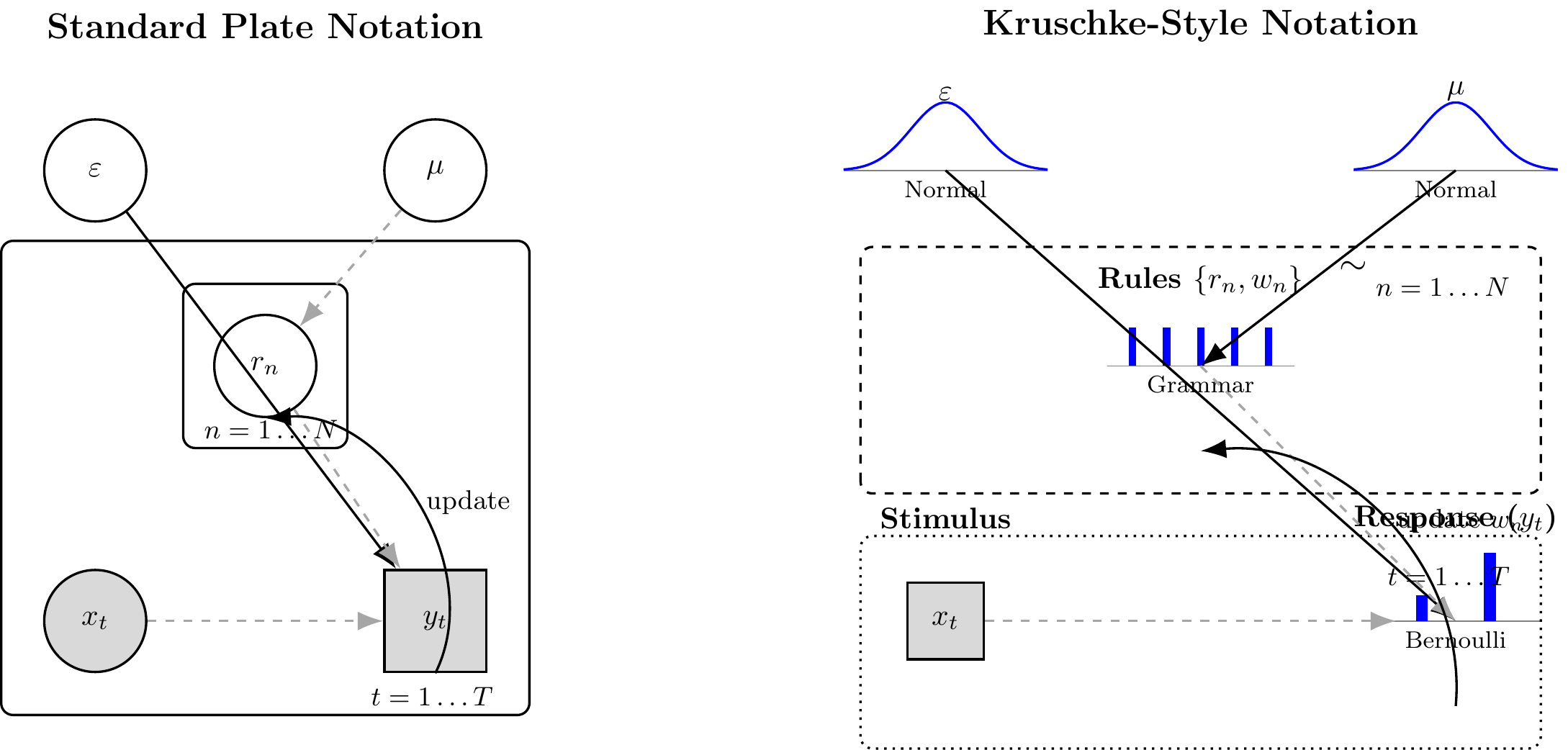
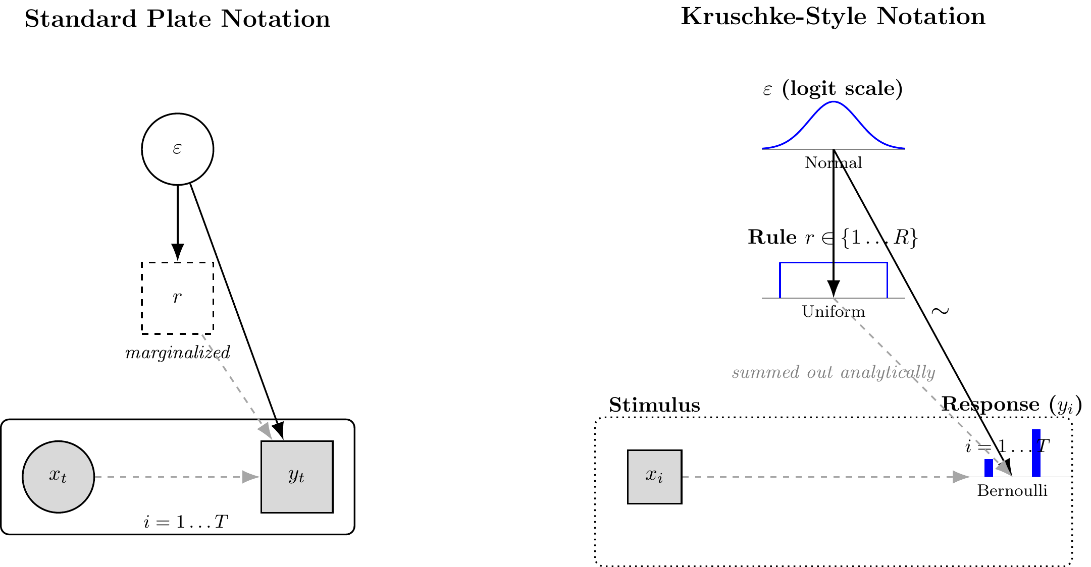
```{tikz ch15_model_a_dag, echo=FALSE, fig.cap="Generative structure of Model A (Bayesian Particle Filter). Left: standard plate notation. Right: Kruschke-style notation. Filled nodes are observed; open nodes are latent. The particle set $\\{r_n\\}$ evolves across trials via resampling and mutation, so the sequential dependency is captured by the trial plate with a self-loop on the particle weights. The two continuous parameters inferred by NPE are $\\varepsilon$ (error probability) and $\\mu$ (mutation probability); $N$ and the rule grammar are fixed structural choices, not estimated.", fig.ext='png', fig.width=12, cache=TRUE}
\usetikzlibrary{positioning, shapes.geometric, arrows.meta, fit, backgrounds, calc}
\tikzset{
stochastic/.style={->, >={Latex[length=3mm]}, thick},
deterministic/.style={->, >={Latex[length=3mm]}, thick, dashed, draw=gray!70},
plate/.style={draw=black, thick, rounded corners, inner sep=10pt},
continuous/.style={circle, draw=black, thick, minimum size=1.2cm, inner sep=0pt},
discrete/.style={rectangle, draw=black, thick, minimum size=1.2cm},
observed/.style={fill=gray!30},
latent/.style={fill=white},
pics/norm_dist/.style={code={
\draw[thin, gray] (-1.2,0) -- (1.2,0);
\draw[thick, blue] plot[domain=-1.2:1.2, samples=50] (\x, {0.8*exp(-3*\x*\x)});
\node[font=\footnotesize, below] at (0,0) {Normal};
}},
pics/bern_dist/.style={code={
\draw[thin, gray] (-1,0) -- (1,0);
\draw[blue, line width=4pt] (-0.4, 0) -- (-0.4, 0.3);
\draw[blue, line width=4pt] (0.4, 0) -- (0.4, 0.8);
\node[font=\footnotesize, below] at (0,0) {Bernoulli};
}},
pics/grammar_dist/.style={code={
\draw[thin, gray] (-1.1,0) -- (1.1,0);
\foreach \x in {-0.8,-0.4,0,0.4,0.8} {
\draw[blue, line width=2.5pt] (\x, 0) -- (\x, 0.45);
}
\node[font=\footnotesize, below] at (0,0) {Grammar};
}}
}
\begin{tikzpicture}
%% LEFT: STANDARD PLATE NOTATION
\node[font=\large\bfseries] at (0, 3.5) {Standard Plate Notation};
% Hyperparameters / priors (fixed structural choices at top)
\node[continuous, latent] (eps) at (-2, 1.8) {$\varepsilon$};
\node[continuous, latent] (mu) at ( 2, 1.8) {$\mu$};
% Particle plate
\node[continuous, latent] (r_n) at (0, -0.5) {$r_n$};
\node[plate, fit=(r_n), label={[anchor=south east, font=\small\bfseries]below right:$n=1\dots N$}] (pN) {};
% Trial plate
\node[continuous, observed] (x_t) at (-2, -3.5) {$x_t$};
\node[discrete, observed] (y_t) at ( 2, -3.5) {$y_t$};
\node[plate, inner sep=14pt, fit=(x_t)(y_t)(pN), label={[anchor=south east, font=\small\bfseries]below right:$t=1\dots T$}] (pT) {};
% Arrows
\draw[stochastic] (eps) -- (y_t);
\draw[deterministic] (mu) -- (r_n);
\draw[deterministic] (r_n) -- (y_t);
\draw[deterministic] (x_t) -- (y_t);
% Self-loop indicating sequential update of particles across trials
\draw[stochastic, bend right=60] (y_t.south) to node[right, font=\small]{update} (r_n.south);
%% RIGHT: KRUSCHKE-STYLE NOTATION
\node[font=\large\bfseries] at (11, 3.5) {Kruschke-Style Notation};
% Priors
\coordinate (k_eps) at (8, 1.8); \draw (k_eps) pic {norm_dist};
\node[above=0.7cm of k_eps, font=\bfseries] {$\varepsilon$};
\coordinate (k_mu) at (14, 1.8); \draw (k_mu) pic {norm_dist};
\node[above=0.7cm of k_mu, font=\bfseries] {$\mu$};
% Particle set (grammar prior)
\coordinate (k_r) at (11, -0.5); \draw (k_r) pic {grammar_dist};
\node[above=0.7cm of k_r, font=\bfseries, align=center] {Rules $\{r_n, w_n\}$};
% Observed stimulus (fixed/given)
\node[discrete, observed, minimum size=0.9cm] (k_x) at (8, -3.5) {$x_t$};
\node[above=0.5cm of k_x, font=\bfseries] {Stimulus};
% Response
\coordinate (k_y) at (14, -3.5); \draw (k_y) pic {bern_dist};
\node[above=0.9cm of k_y, font=\bfseries] {Response ($y_t$)};
% Plates
\draw[plate, dashed] (7.0, -2.0) rectangle (15.0, 0.9) node[below left, font=\small\bfseries] {$n=1\dots N$};
\draw[plate, dotted] (7.0, -5.0) rectangle (15.0, -2.5) node[below left, font=\small\bfseries] {$t=1\dots T$};
% Arrows
\draw[stochastic] (k_eps) -- (k_y);
\draw[stochastic] (k_mu) -- (k_r) node[midway, right, font=\large]{$\sim$};
\draw[deterministic] (k_r) -- (k_y);
\draw[deterministic] (k_x) -- (13.3, -3.5);
% Sequential update arrow
\draw[stochastic, bend right=50] (14, -4.5) to node[right, font=\small]{update $w_n$} (11, -1.5);
\end{tikzpicture}
```
### Why Model A's Likelihood is Intractable for HMC
Stan's HMC sampler requires a continuous, differentiable log posterior density. Individual rule particles are discrete, symbolic structures — lists containing integers, operators, and real-valued thresholds. The *space* of all possible rules is a combinatorial set of structured objects: there is no natural notion of a gradient with respect to "which logical operator appears in condition 1" or "which dimension is used." This is exactly the class of discrete latent variables that must be integrated out analytically before any Stan code is written (the same principle we applied to mixture components in Chapter 8).
For Model A, this analytical marginalisation is **not feasible in closed form** over a combinatorial rule space crossed with continuous thresholds and a non-differentiable resampling step. The particle filter therefore lives entirely in R, where it acts as its own approximate Bayesian inference engine via sequential Monte Carlo.
**This is the standard situation for which simulator-based inference was invented.** The Lintusaari et al. ABC review describes the pattern exactly:
> "Many recent models in biology describe nature to a high degree of accuracy but are not amenable to analytical treatment. The models can, however, be simulated on computers… While it is usually relatively easy to generate data from the models for any configuration of the parameters, the real interest is often focused on the inverse problem: the identification of parameter configurations that would plausibly lead to data that are sufficiently similar to the observed data."
Model A is exactly such a model: $\theta = (\varepsilon, N_{\text{particles}}, \text{max\_dims}, \ldots)$, $V$ is the random variables driving particle initialisation and resampling, $M$ is the `rule_particle_filter` function, and $y$ is the trial-by-trial response sequence. Section "Neural Posterior Estimation for Model A" implements NPE for this simulator. Until then, we treat the particle filter purely as a forward simulator.
### Parameters: Cognitive Commitment, Algebraic Role, NPE Parameterization
| Parameter | Cognitive meaning | Algebraic role | R / NPE parameterization |
|---|---|---|---|
| **ε** (error prob) | Probability that a learner misapplies an otherwise-correct rule; captures lapses, feature noise, and decision variability | Softens the weighted particle vote: $\hat{p}_t = \sum_n w_n [(1-\varepsilon)\,\mathbf{1}_{\{r_n=1\}} + \varepsilon\,\mathbf{1}_{\{r_n=0\}}]$ | `error_prob` in `rule_particle_filter()`; inferred on the logit scale: `logit(ε) ~ Normal(0, 1.5)` |
| **μ** (mutation rate) | Per-trial probability that a learner discards the current hypothesis and draws a fresh one from the grammar; controls how readily rules are revised | Drives hypothesis diversity after resampling: each particle independently replaced by $r_n^{\text{new}} \sim p_{\mathcal{R}}$ with probability $\mu$ | `mutation_prob` in `rule_particle_filter()`; inferred on the logit scale: `logit(μ) ~ Normal(-3, 1.5)` |
| **N** (particles) | Working-memory capacity: number of rule hypotheses the learner maintains simultaneously | Controls approximation quality of the SMC filter; not a continuous parameter — a structural commitment | Fixed at `N_PARTICLES_FIXED = 100`; treated as a sensitivity variable in §"Sensitivity to Rule-Set Size" |
**Trilogy comparison.** ε is the rule-model analogue of the GCM's sensitivity $c$ (sharpness of evidence accumulation) and the prototype model's $\sigma$ (response noise). μ is the analogue of the decay GCM's forgetting rate $\lambda$ and the Kalman prototype's process noise $q$ — the parameter that allows the model to track non-stationary categories.
### Mathematical Formulation
Model A is a state-space generative model. Let $N$ denote the number of particles, $\mathcal{R}$ the rule grammar, and $\varepsilon, \mu \in (0,1)$ the error and mutation probabilities.
**Priors:**
$$\text{logit}(\varepsilon) \sim \mathcal{N}(0,\ 1.5) \qquad \text{logit}(\mu) \sim \mathcal{N}(-3,\ 1.5)$$
**Initialisation** ($t = 0$): draw $N$ rules i.i.d. from the grammar prior, $r_n^{(0)} \sim p_{\mathcal{R}}$; set weights $w_n^{(0)} = 1/N$.
**Per-trial update** (for trial $t = 1, \ldots, T$, stimulus $\mathbf{x}_t$, label $y_t \in \{0,1\}$):
1. **Predict:** $\hat{p}_t = \sum_{n=1}^{N} w_n^{(t-1)} \cdot \left[(1-\varepsilon)\,\mathbf{1}\{r_n \text{ predicts } 1\} + \varepsilon\,\mathbf{1}\{r_n \text{ predicts } 0\}\right]$
2. **Weight update:** $\tilde{w}_n^{(t)} \propto w_n^{(t-1)} \cdot \left[(1-\varepsilon)^{\mathbf{1}\{r_n(\mathbf{x}_t)=y_t\}} \cdot \varepsilon^{\mathbf{1}\{r_n(\mathbf{x}_t)\neq y_t\}}\right]$
3. **Resample** if $\text{ESS} = 1/\sum_n (\tilde{w}_n^{(t)})^2 < N/2$: draw indices with replacement proportional to $\tilde{w}_n^{(t)}$; reset weights to $1/N$.
4. **Mutate:** each particle independently replaced by $r_n^{\text{new}} \sim p_{\mathcal{R}}$ with probability $\mu$.
5. **Observe:** $y_t \mid \hat{p}_t \sim \text{Bernoulli}(\hat{p}_t)$.
The resampling step in (3) is non-differentiable, which means the marginal likelihood $p(\mathbf{y} \mid \varepsilon, \mu)$ has no closed form and HMC cannot be applied. The steps below walk through each operation in detail and supply the R helper functions that the full agent assembles.
#### Step 1: Generating Initial Rule Particles
```{r ch15_generate_rules}
# Generate a single random rule.
# This is the implementation of the formal grammar from §"Rule Grammar".
generate_random_rule <- function(n_features,
                                 max_dims      = MAX_RULE_DIMS,
                                 feature_range = list(c(0, 5), c(0, 5)),
                                 nested_prob   = 0.25) {
  # With probability nested_prob, generate a nested 3-condition rule (if
  # there are >= 2 features and the grammar allows it). Otherwise generate
  # a flat 1- or 2-condition rule as before.
  use_nested <- (n_features >= 2) && (runif(1) < nested_prob)

  sample_thresh <- function(di) runif(1, feature_range[[di]][1], feature_range[[di]][2])

  if (use_nested) {
    # Three conditions; dimensions may repeat (same feature, different thresholds)
    dims_used  <- sample(seq_len(n_features), size = 3, replace = TRUE)
    thresholds <- mapply(sample_thresh, dims_used)
    operations <- sample(RULE_OPERATORS, 3, replace = TRUE)
    list(
      dimensions         = dims_used,
      thresholds         = thresholds,
      operations         = operations,
      outer_logic        = sample(RULE_LOGIC, 1),
      inner_logic        = sample(RULE_LOGIC, 1),
      prediction_if_true = sample(0:1, 1)
    )
  } else {
    num_dims  <- sample(seq_len(min(max_dims, n_features)), 1)
    dims_used <- sort(sample(seq_len(n_features), size = num_dims, replace = FALSE))
    thresholds <- numeric(num_dims)
    operations <- character(num_dims)
    for (k in seq_len(num_dims)) {
      di            <- dims_used[k]
      thresholds[k] <- sample_thresh(di)
      operations[k] <- sample(RULE_OPERATORS, 1)
    }
    list(
      dimensions        = dims_used,
      thresholds        = thresholds,
      operations        = operations,
      logic             = if (num_dims == 2) sample(RULE_LOGIC, 1) else NA,
      prediction_if_true = sample(0:1, 1)
    )
  }
}

# Initialize N particles with equal weights.
initialize_particles <- function(n_particles, n_features,
                                  max_dims = MAX_RULE_DIMS,
                                  feature_range = list(c(0, 5), c(0, 5))) {
  particles <- vector("list", n_particles)
  for (i in seq_len(n_particles))
    particles[[i]] <- generate_random_rule(n_features, max_dims, feature_range)
  list(particles = particles, weights = rep(1 / n_particles, n_particles))
}

# --- Example ---
n_particles_example <- 5
n_features_example  <- 2
initial_system <- initialize_particles(n_particles_example, n_features_example)
cat(paste("Initialized", n_particles_example, "particles. Example rule 1:\n"))
print(initial_system$particles[[1]])
cat("Initial weights:", initial_system$weights, "\n")
```
#### Step 2: Updating Particle Weights
When we observe a stimulus $\vec{x}$ and its true category $y$, we update weight $w_i$ for each particle $i$. We introduce a small $\varepsilon$ (`error_prob`) to allow for occasional noise or misapplication:
$$P(y \mid \vec{x}, \text{rule}_i) = \begin{cases} 1 - \varepsilon & \text{if rule}_i \text{ predicts } y \\ \varepsilon & \text{otherwise} \end{cases}$$
The updated weight is $w_i' \propto w_i \times P(y \mid \vec{x}, \text{rule}_i)$, then renormalized.
```{r ch15_update_weights}
update_weights <- function(particles, weights, stimulus, true_category,
                           error_prob = 0.05) {
  n <- length(particles)
  new_w <- numeric(n)
  for (i in seq_len(n)) {
    pred      <- evaluate_rule(particles[[i]], stimulus)
    likelihood <- if (pred == true_category) 1 - error_prob else error_prob
    new_w[i]  <- weights[i] * likelihood
  }
  total <- sum(new_w)
  if (total > 1e-9) new_w / total else rep(1 / n, n)
}

# --- Example ---
cat("\n--- Example Weight Update ---\n")
updated_w <- update_weights(
  initial_system$particles, initial_system$weights,
  stimulus = c(4, 3), true_category = 1, error_prob = 0.1
)
preds <- sapply(initial_system$particles, evaluate_rule, stimulus = c(4, 3))
cat("Rule predictions for stimulus [4, 3]:", preds, "\n")
cat("Weights BEFORE:", round(initial_system$weights, 3), "\n")
cat("Weights AFTER: ", round(updated_w, 3), "\n")
```
#### Step 3: Resampling Particles
If we only update weights, eventually most weights become near zero and only a few particles dominate — **particle degeneracy**. Resampling revitalizes the particle set by drawing $N$ new particles with probability proportional to weights, then resetting all weights to $1/N$.
**Why not resample when any individual weight falls below a threshold?** A single low weight is not a reliable signal: in a healthy filter, a few particles always receive less support than the rest. A per-particle threshold triggers resampling whenever one particle becomes unlikely — which can happen after every informative trial even when the overall set is perfectly adequate. The result is constant, unnecessary resampling that destroys diversity without solving any real problem. The relevant question is not "is any single weight small?" but "how much of the population is effectively pulling its weight?"
**Why not resample on every trial?** Resampling discards particles: particles that lose a draw at one step may have been the correct hypothesis a few trials later, after an unexpected observation. Resampling every trial collapses diversity prematurely and makes the filter brittle to any short streak of misleading feedback. It also breaks the sequential importance-sampling interpretation of the filter — the weights are supposed to accumulate evidence across trials before being acted on.
**The ESS-based threshold balances both concerns.** The **Effective Sample Size** $\text{ESS} = 1 / \sum_i w_i^2$ is a single number that summarises the whole weight distribution: it equals $N$ when all weights are uniform (maximum diversity) and approaches 1 when one particle has all the weight (complete degeneracy). Using the rule "resample when $\text{ESS} < N \times \tau$" (with $\tau = 0.5$ as the default threshold) means resampling fires only when the collective distribution of weights has become concentrated — not because any particular particle is small, and not on a fixed schedule. This allows weights to accumulate evidence across trials when the current hypothesis set is still informative, and intervenes only when the approximation quality has genuinely degraded.
> **A note on ESS here vs. ESS in MCMC diagnostics.** ESS appears in two distinct contexts in this book. In Chapters 4–10 it measures how many effectively independent posterior draws an MCMC chain produces, diagnosing autocorrelation. Here it measures how many particles are effectively contributing to the filter's approximation, given their weights. Both are measures of statistical efficiency under a sampling procedure — the underlying intuition (fewer effective units = less reliable estimate) is the same — but the contexts are different. The MCMC ESS is about temporal autocorrelation; the particle ESS is about weight concentration. Both names are correct and they refer to genuinely different things.
```{r ch15_resample_particles}
resample_particles <- function(particles, weights) {
  n          <- length(particles)
  idx        <- sample.int(n, size = n, replace = TRUE, prob = weights)
  new_p      <- particles[idx]
  new_w      <- rep(1 / n, n)
  list(particles = new_p, weights = new_w)
}

# --- Example ---
cat("\n--- Example Resampling ---\n")
skewed_w <- c(0.01, 0.60, 0.02, 0.35, 0.02)
cat("Weights BEFORE resampling:", skewed_w, "\n")
rs <- resample_particles(initial_system$particles, skewed_w)
cat("Weights AFTER resampling: ", rs$weights, "\n")
```
#### Step 4: Mutating Particles
Resampling solves particle degeneracy but creates a subtler problem: the effective hypothesis space shrinks monotonically. Every particle that loses the resampling lottery is gone forever, and no new rules are ever introduced. A filter running long enough on any task will collapse to a handful of particles — possibly the right ones, but with no ability to recover if the task changes or if the true rule was simply unlucky at initialisation.
The mutation step is the direct fix: after resampling on each trial, each particle independently regenerates with probability $\mu$, replaced by a fresh rule drawn from the grammar. The parameter $\mu$ is the third free parameter of Model A (alongside $\varepsilon$ and the structural commitments). It plays the same conceptual role as process noise $q$ in the Kalman prototype and forgetting rate $\lambda$ in the decay GCM:
| Chapter | Model | Non-stationarity parameter | Mechanism |
|---|---|---|---|
| Ch. 13 (decay GCM) | Exemplar store | $\lambda$ (forgetting rate) | Exponentially downweight old exemplars |
| Ch. 14 (Kalman prototype) | Running mean + covariance | $q$ (process noise) | Re-inflate uncertainty each trial |
| Ch. 15 (rule filter) | Particle distribution over rules | $\mu$ (mutation rate) | Randomly regenerate a fraction of particles each trial |
Setting $\mu = 0$ recovers a pure selection filter. On a stationary task, small $\mu$ barely affects inference — the filter mostly selects and the occasional regenerated particle is usually wrong, so it is quickly downweighted. On a task where the correct rule changes, $\mu > 0$ is essential: without it, all the rules that would fit the new regime have been eliminated and the filter cannot recover.
```{r ch15_rule_mutation}
# At each trial, each particle independently has probability mutation_prob
# of being replaced by a freshly drawn rule from the grammar.
# mutation_prob = 0 is a no-op (pure selection filter).
mutate_particles <- function(particles, mutation_prob, n_features,
                             max_dims, feature_range) {
  if (mutation_prob <= 0) return(particles)
  n <- length(particles)
  to_mutate <- which(runif(n) < mutation_prob)
  for (i in to_mutate) {
    particles[[i]] <- generate_random_rule(n_features, max_dims, feature_range)
  }
  particles
}
```
This is the **prior-sampling** mutation kernel: replacement rules are drawn uniformly from the grammar, with no relationship to the rule they replace. §"Targeted Mutation: Revision Rather Than Replacement" develops cognitively motivated alternatives where the learner *revises* rather than discards — keeping useful features and adjusting only what failed.
#### Step 5: Making Predictions
The particle filter makes a categorization decision for a new stimulus $\vec{x}$ via a weighted vote across all particles:
$$P(\text{Choose Cat 1} \mid \vec{x}) = \sum_{i=1}^{N} w_i \times P(\text{Cat 1} \mid \vec{x}, \text{rule}_i)$$
where $P(\text{Cat 1} \mid \vec{x}, \text{rule}_i) = 1 - \varepsilon$ if rule $i$ predicts category 1, and $\varepsilon$ otherwise.
### R Implementation of the Particle Filter Agent
```{r ch15_particle_filter_agent}
# Full particle filter agent — this is Model A.
# Returns a tibble of prob_cat1 and sim_response for each trial.
# Note: n_particles defaults to N_PARTICLES_FIXED (= 100), the structural
# structural commitment documented in §"Rule Grammar: Formal Specification".
rule_particle_filter <- function(n_particles               = N_PARTICLES_FIXED,
                                 error_prob,
                                 mutation_prob             = 0.0,
                                 obs,
                                 cat_one,
                                 max_dims                  = MAX_RULE_DIMS,
                                 resample_threshold_factor = RESAMPLE_THRESHOLD,
                                 quiet                     = TRUE) {
  n_trials   <- nrow(obs)
  n_features <- ncol(obs)
  # feature_range is built generically across n_features so the same simulator
  # handles 2D continuous (Kruschke) and 5D binary (Ch. 16 Alien Game) inputs.
  fr         <- lapply(seq_len(n_features), function(d) range(obs[, d]))

  ps        <- initialize_particles(n_particles, n_features, max_dims, fr)
  particles <- ps$particles
  weights   <- ps$weights

  response_probs <- numeric(n_trials)

  for (i in seq_len(n_trials)) {
    if (!quiet && i %% 20 == 0) cat("Trial", i, "\n")

    stim <- as.numeric(obs[i, ])

    # ── Prediction ────────────────────────────────────────────────────────────
    preds        <- sapply(particles, evaluate_rule, stimulus = stim)
    p_cat1_rules <- ifelse(preds == 1, 1 - error_prob, error_prob)
    p            <- sum(weights * p_cat1_rules)
    response_probs[i] <- pmax(1e-9, pmin(1 - 1e-9, p))

    # ── Weight update ─────────────────────────────────────────────────────────
    weights <- update_weights(particles, weights, stim, cat_one[i], error_prob)

    # ── Resample if ESS is low ────────────────────────────────────────────────
    ess <- 1 / sum(weights^2)
    if (ess < n_particles * resample_threshold_factor) {
      rs        <- resample_particles(particles, weights)
      particles <- rs$particles
      weights   <- rs$weights
    }

    # ── Mutation ──────────────────────────────────────────────────────────────
    # After resampling, each particle independently regenerates with probability
    # mutation_prob. mutation_prob = 0 is a no-op (pure selection filter).
    particles <- mutate_particles(particles, mutation_prob, n_features,
                                  max_dims, fr)
  }

  tibble(prob_cat1 = response_probs,
         sim_response = rbinom(n_trials, 1, response_probs))
}

cat("Particle filter agent function defined.\n")
```
This implementation captures the core cognitive processes hypothesized by rule-based models: hypothesis generation, testing against evidence, belief updating, and adaptive focusing of the hypothesis set. **It is also the simulator that NPE will use in §"Neural Posterior Estimation for Model A."**
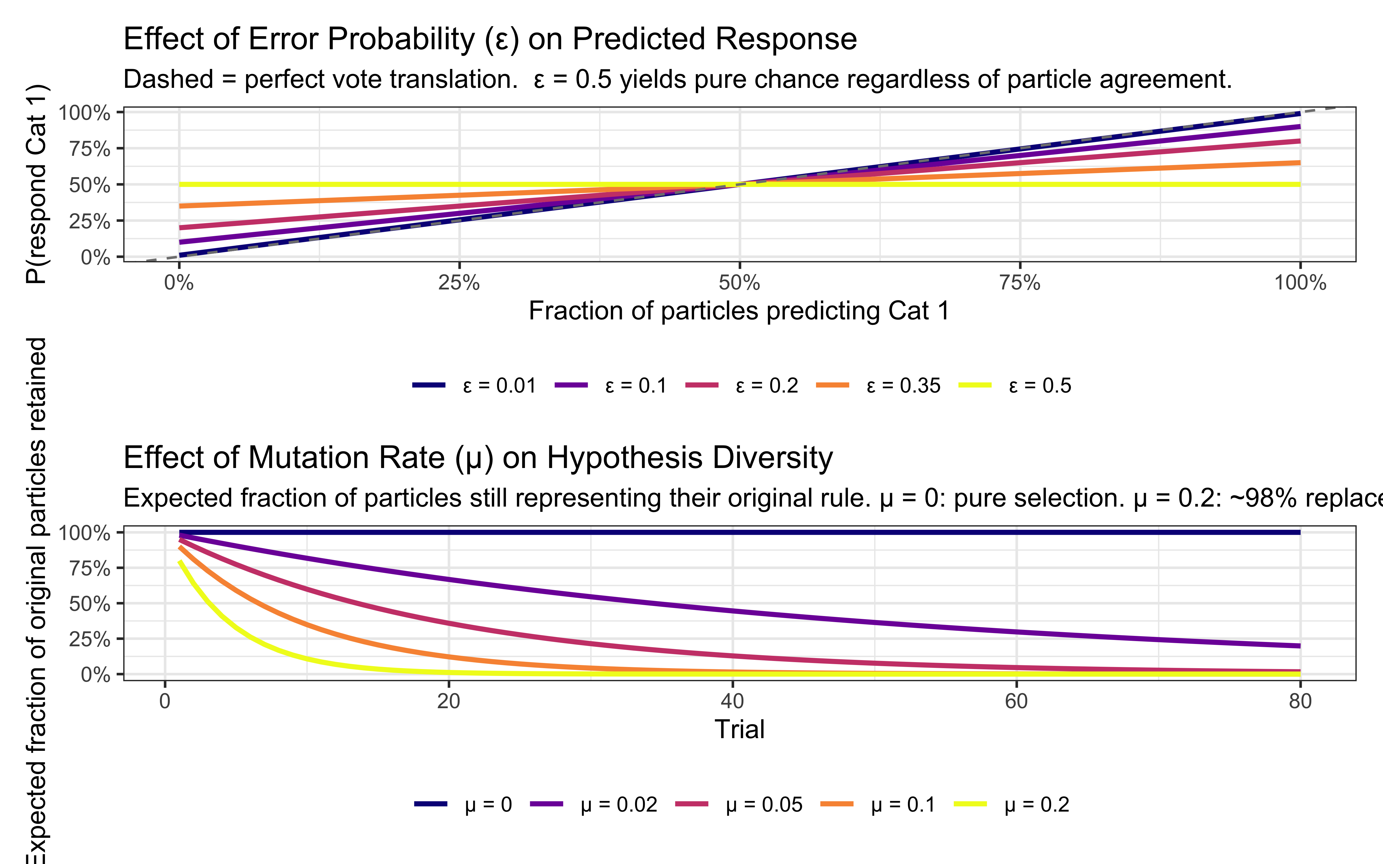
### Visualizing the Effect of ε and μ
Before running full simulations it is worth seeing what the two continuous parameters *do* mathematically — the same exercise performed for sensitivity $c$ in Chapter 11.
```{r ch15_param_effects}
# ── ε panel: how error probability softens the particle vote ─────────────────
eps_df <- expand_grid(
  frac_correct = seq(0, 1, by = 0.01),
  eps          = c(0.01, 0.10, 0.20, 0.35, 0.50)
) |>
  mutate(
    p_cat1    = frac_correct * (1 - eps) + (1 - frac_correct) * eps,
    eps_label = factor(eps, labels = paste0("ε = ", c(0.01, 0.10, 0.20, 0.35, 0.50)))
  )

p_eps <- ggplot(eps_df, aes(x = frac_correct, y = p_cat1,
                             color = eps_label, group = eps_label)) +
  geom_line(linewidth = 1) +
  geom_abline(slope = 1, intercept = 0, linetype = "dashed", color = "grey50") +
  scale_color_viridis_d(option = "plasma", name = NULL) +
  scale_x_continuous(labels = scales::percent) +
  scale_y_continuous(labels = scales::percent) +
  labs(
    title    = "Effect of Error Probability (ε) on Predicted Response",
    subtitle = "Dashed = perfect vote translation.  ε = 0.5 yields pure chance regardless of particle agreement.",
    x        = "Fraction of particles predicting Cat 1",
    y        = "P(respond Cat 1)"
  ) +
  theme_bw() + theme(legend.position = "bottom")

# ── μ panel: how mutation rate drives hypothesis turnover ────────────────────
mu_df <- expand_grid(
  trial    = 1:80,
  mu       = c(0, 0.02, 0.05, 0.10, 0.20)
) |>
  mutate(
    frac_surviving = (1 - mu)^trial,
    mu_label       = factor(mu, labels = paste0("μ = ", c(0, 0.02, 0.05, 0.10, 0.20)))
  )

p_mu <- ggplot(mu_df, aes(x = trial, y = frac_surviving,
                           color = mu_label, group = mu_label)) +
  geom_line(linewidth = 1) +
  scale_color_viridis_d(option = "plasma", name = NULL) +
  scale_y_continuous(labels = scales::percent, limits = c(0, 1)) +
  labs(
    title    = "Effect of Mutation Rate (μ) on Hypothesis Diversity",
    subtitle = "Expected fraction of particles still representing their original rule. μ = 0: pure selection. μ = 0.2: ~98% replaced by trial 20.",
    x        = "Trial",
    y        = "Expected fraction of original particles retained"
  ) +
  theme_bw() + theme(legend.position = "bottom")

p_eps / p_mu
```
The two panels map directly onto the trilogy comparison: ε controls *response softness* (the analogue of sensitivity $c$ in the GCM and $\sigma$ in the prototype model), while μ controls *hypothesis turnover* (the analogue of forgetting rate $\lambda$ in the decay GCM and process noise $q$ in the Kalman prototype). The key difference from those continuous-state models is that μ acts on a discrete particle set — replacement is all-or-nothing rather than a smooth re-inflation of variance — which is why the fraction curve is exponential rather than linear.
::: {.callout-tip title="Generalization checklist for downstream chapters"}
The `rule_particle_filter` above is written so that the same function body runs unchanged on Chapter 16's 5-feature binary alien stimuli. A downstream chapter inherits the simulator by changing only the four items below — none of which touch the trial loop, the weight update, the resampling step, or the mutation step.
| Item | Kruschke (Ch. 15) | Alien Game (Ch. 16) |
|---|---|---|
| `n_features` | $2$ (height, position) | $5$ (binary feature vector) |
| `feature_range` | per-feature `range(obs[, d])` | `c(0, 1)` per feature |
| Threshold sampling | `runif(1, lo, hi)` | hard-coded at $0.5$ |
| `max_dims` default | $2$ | $3$ |
The grammar object (`dimensions`, `thresholds`, `operations`, `logic` / `outer_logic` / `inner_logic`, `prediction_if_true`) is identical in both chapters; the nested form $A\ L_{\text{outer}}\ (B\ L_{\text{inner}}\ C)$ is preserved so the alien-game grammar `A AND (B OR C)` is directly representable.
:::
---
## Simulating Categorization Behavior
Let's simulate how Model A performs on the Kruschke (1993) task. Each agent receives its **own independently randomized stimulus order**, consistent with the path-dependence design from Chapters 11 and 12.
```{r ch15_simulate_rule_responses}
# Wrapper: generates per-agent schedule then calls rule_particle_filter.
simulate_rule_agent <- function(agent_id, n_particles, max_dims, error_prob,
                                stimulus_info, n_blocks, subject_seed,
                                mutation_prob = 0.0) {
  schedule <- make_subject_schedule(stimulus_info, n_blocks, seed = subject_seed)
  obs      <- as.matrix(schedule[, c("height", "position")])
  cat_one  <- schedule$category_feedback

  result <- rule_particle_filter(
    n_particles               = n_particles,
    error_prob                = error_prob,
    mutation_prob             = mutation_prob,
    obs                       = obs,
    cat_one                   = cat_one,
    max_dims                  = max_dims,
    resample_threshold_factor = RESAMPLE_THRESHOLD,
    quiet                     = TRUE
  )

  schedule |>
    mutate(
      agent_id      = agent_id,
      n_particles   = n_particles,
      max_dims      = max_dims,
      error_prob    = error_prob,
      mutation_prob = mutation_prob,
      prob_cat1     = result$prob_cat1,
      sim_response  = result$sim_response,
      correct       = as.integer(category_feedback == sim_response)
    ) |>
    group_by(agent_id, n_particles, max_dims, error_prob, mutation_prob) |>
    mutate(performance = slider::slide_dbl(correct, mean, .before = 4, .complete = TRUE)) |>
    ungroup()
}

param_df_rules <- expand_grid(
  agent_id    = 1:10,
  n_particles = c(50, 200),         # exploring sensitivity to N_particles
  max_dims    = c(1, 2),            # exploring sensitivity to grammar depth
  error_prob  = c(0.05, 0.2)
) |>
  mutate(subject_seed = agent_id)   # unique, reproducible seed per agent

rule_sim_file <- here("simdata", "ch14_rule_simulated_responses.csv")

if (regenerate_simulations || !file.exists(rule_sim_file)) {
  cat("Regenerating rule-based simulations...\n")
  rule_responses <- future_pmap_dfr(
    list(
      agent_id    = param_df_rules$agent_id,
      n_particles = param_df_rules$n_particles,
      max_dims    = param_df_rules$max_dims,
      error_prob  = param_df_rules$error_prob,
      subject_seed = param_df_rules$subject_seed
    ),
    simulate_rule_agent,
    stimulus_info = stimulus_info,
    n_blocks      = n_blocks,
    .options = furrr_options(seed = TRUE)
  )
  write_csv(rule_responses, rule_sim_file)
  cat("Simulations saved.\n")
} else {
  rule_responses <- read_csv(rule_sim_file, show_col_types = FALSE)
  cat("Simulations loaded.\n")
}
ggplot(rule_responses,
       aes(x = trial_within_subject, y = performance,
           color = factor(n_particles))) +
  stat_summary(fun = mean, geom = "line", linewidth = 1) +
  stat_summary(fun.data = mean_se, geom = "ribbon", alpha = 0.15,
               aes(fill = factor(n_particles)), linetype = 0) +
  facet_grid(
    max_dims ~ error_prob,
    labeller = labeller(
      max_dims   = function(x) paste("Max Dims:", x),
      error_prob = function(x) paste("Error Prob:", x)
    )
  ) +
  scale_color_viridis_d(option = "plasma", name = "N Particles") +
  scale_fill_viridis_d(option = "plasma", name = "N Particles") +
  labs(
    title    = "Rule-Based Model Learning Performance (Model A)",
    subtitle = "Facets show effect of max rule dimensions and error probability",
    x = "Trial", y = "Rolling Accuracy — 5-trial window (Mean ± SE)"
  ) +
  ylim(0.4, 1.0)
```
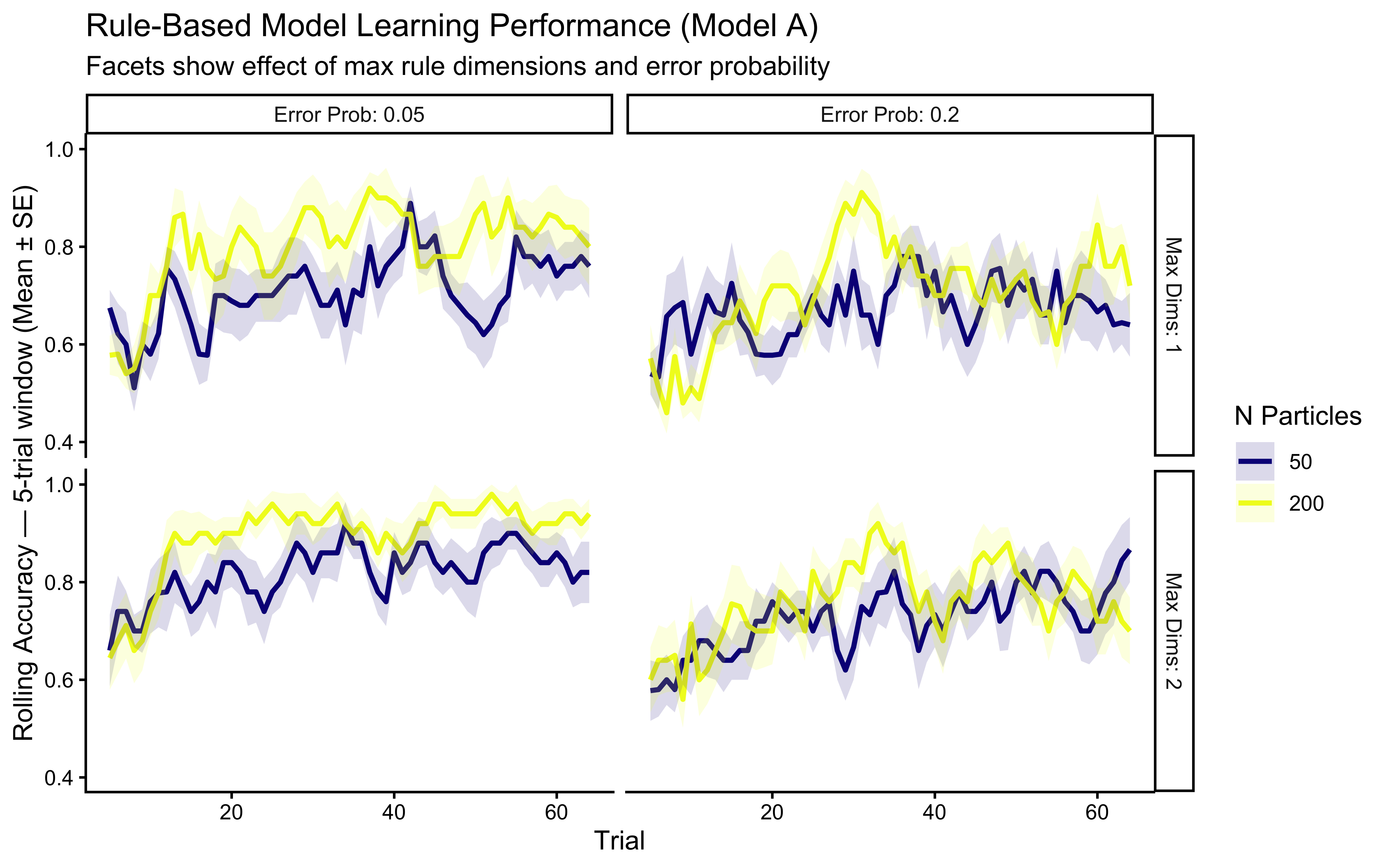
**Simulation Interpretation**: This visualization shows how Model A's performance is affected by:
* **Number of Particles**: More particles allow better exploration of the rule space, potentially leading to faster learning or higher final accuracy, though gains may diminish. **This parameter has cognitive content** (working-memory bound on hypothesis count) and is a candidate for NPE inference rather than fixing.
* **Maximum Rule Dimensions**: Allowing 2D rules (`max_dims = 2`) may be necessary if the true category boundary requires integrating information across dimensions. Setting `max_dims = 1` corresponds to a simpler grammar that cannot express conjunctive concepts.
* **Error Probability**: A higher `error_prob` makes the model more tolerant of imperfect rules, which can be helpful in noisy environments but may prevent convergence on a precise rule if one exists.
### Visualizing Rule Learning Over Time
A key feature of Model A is that the hypotheses are explicit. We can track which rules the particle filter believes are most likely at different points during learning.
```{r ch15_track_rule_learning}
track_rule_learning <- function(n_particles, error_prob, obs, cat_one,
                                mutation_prob             = 0.0,
                                max_dims                  = MAX_RULE_DIMS,
                                top_k                     = 1,
                                resample_threshold_factor = RESAMPLE_THRESHOLD) {
  n_trials  <- nrow(obs)
  n_features <- ncol(obs)
  fr         <- lapply(seq_len(n_features), function(d) range(obs[, d]))

  ps        <- initialize_particles(n_particles, n_features, max_dims, fr)
  particles <- ps$particles
  weights   <- ps$weights

  format_rule_info <- function(rule) {
    list(
      dimension1  = if (length(rule$dimensions) >= 1) rule$dimensions[1] else NA_integer_,
      operation1  = if (length(rule$operations)  >= 1) rule$operations[1]  else NA_character_,
      threshold1  = if (length(rule$thresholds)  >= 1) rule$thresholds[1]  else NA_real_,
      dimension2  = if (length(rule$dimensions) >= 2) rule$dimensions[2] else NA_integer_,
      operation2  = if (length(rule$operations)  >= 2) rule$operations[2]  else NA_character_,
      threshold2  = if (length(rule$thresholds)  >= 2) rule$thresholds[2]  else NA_real_,
      dimension3  = if (length(rule$dimensions) >= 3) rule$dimensions[3] else NA_integer_,
      operation3  = if (length(rule$operations)  >= 3) rule$operations[3]  else NA_character_,
      threshold3  = if (length(rule$thresholds)  >= 3) rule$thresholds[3]  else NA_real_,
      logic       = if (!is.null(rule$logic)) rule$logic
                    else if (!is.null(rule$outer_logic)) paste0(rule$outer_logic, "(", rule$inner_logic, ")")
                    else "N/A",
      prediction  = rule$prediction_if_true
    )
  }

  history <- vector("list", n_trials)
  for (i in seq_len(n_trials)) {
    stim    <- as.numeric(obs[i, ])
    weights <- update_weights(particles, weights, stim, cat_one[i], error_prob)

    top_idx <- order(weights, decreasing = TRUE)[seq_len(min(top_k, n_particles))]
    history[[i]] <- map_dfr(top_idx, ~{
      tibble(trial = i, rank = which(top_idx == .x),
             weight = weights[.x], !!!format_rule_info(particles[[.x]]))
    })

    ess <- 1 / sum(weights^2)
    if (ess < n_particles * resample_threshold_factor) {
      rs        <- resample_particles(particles, weights)
      particles <- rs$particles
      weights   <- rs$weights
    }

    particles <- mutate_particles(particles, mutation_prob, n_features,
                                  max_dims, fr)
  }
  bind_rows(history)
}

# Run tracking with a fixed seed-1 schedule for reproducibility
track_schedule <- make_subject_schedule(stimulus_info, n_blocks, seed = 1)

rule_tracking_data <- track_rule_learning(
  n_particles   = N_PARTICLES_FIXED,
  error_prob    = 0.1,
  mutation_prob = plogis(LOGIT_MU_PRIOR_MEAN),   # prior median ≈ 0.047
  obs           = as.matrix(track_schedule[, c("height", "position")]),
  cat_one       = track_schedule$category_feedback,
  max_dims      = MAX_RULE_DIMS,
  top_k         = 1
)

# Format rule text for plotting
rule_to_text <- function(rule_row) {
  dim_names <- c("Height", "Position")
  if (is.na(rule_row$dimension2)) {
    sprintf("IF %s %s %.1f THEN Cat %d",
            dim_names[rule_row$dimension1], rule_row$operation1,
            rule_row$threshold1, rule_row$prediction)
  } else {
    sprintf("IF %s %s %.1f %s %s %s %.1f THEN Cat %d",
            dim_names[rule_row$dimension1], rule_row$operation1, rule_row$threshold1,
            rule_row$logic,
            dim_names[rule_row$dimension2], rule_row$operation2, rule_row$threshold2,
            rule_row$prediction)
  }
}

rule_tracking_plot_data <- rule_tracking_data |>
  filter(rank == 1) |>
  rowwise() |>
  mutate(rule_text = rule_to_text(cur_data())) |>
  ungroup() |>
  mutate(rule_block = consecutive_id(rule_text))

# Vertical lines at every hypothesis switch
rule_switches <- rule_tracking_plot_data |>
  group_by(rule_block) |>
  summarise(switch_trial = min(trial), .groups = "drop") |>
  filter(switch_trial > 1)

# Label only the top-4 highest-weight peaks (most informative moments)
top_labels <- rule_tracking_plot_data |>
  group_by(rule_block, rule_text) |>
  slice_max(weight, n = 1, with_ties = FALSE) |>
  ungroup() |>
  slice_max(weight, n = 4) |>
  mutate(rule_text = str_wrap(rule_text, width = 30))

# Run particle filter on the same schedule to get trial-by-trial responses
set.seed(1)
track_filter <- rule_particle_filter(
  n_particles   = N_PARTICLES_FIXED,
  error_prob    = 0.1,
  mutation_prob = plogis(LOGIT_MU_PRIOR_MEAN),
  obs           = as.matrix(track_schedule[, c("height", "position")]),
  cat_one       = track_schedule$category_feedback,
  max_dims      = MAX_RULE_DIMS,
  quiet         = TRUE
)

track_perf <- tibble(
  trial   = seq_len(nrow(track_schedule)),
  correct = as.integer(track_filter$sim_response == track_schedule$category_feedback)
) |>
  mutate(rolling_acc = slider::slide_dbl(correct, mean, .before = 4, .complete = TRUE))

p_weights <- ggplot(rule_tracking_plot_data, aes(x = trial, y = weight)) +
  geom_vline(
    data = rule_switches, aes(xintercept = switch_trial - 0.5),
    linetype = "dashed", color = "grey60", linewidth = 0.4
  ) +
  geom_line(aes(group = 1), color = "#0072B2") +
  geom_point(color = "#0072B2", size = 1.5) +
  geom_text_repel(
    data = top_labels,
    aes(label = rule_text),
    size = 2.8, lineheight = 0.9,
    box.padding = 0.5, point.padding = 0.3,
    max.overlaps = Inf, min.segment.length = 0
  ) +
  scale_y_continuous(limits = c(0, NA), name = "Weight of Top Rule") +
  scale_x_continuous(limits = c(0, total_trials + 5)) +
  labs(
    title    = "Evolution of the Top Rule Hypothesis Over Time (Model A)",
    subtitle = "Dashed lines mark hypothesis switches; labels show the four highest-weight rules.",
    x = NULL
  )

p_perf <- ggplot(track_perf, aes(x = trial, y = rolling_acc)) +
  geom_vline(
    data = rule_switches, aes(xintercept = switch_trial - 0.5),
    linetype = "dashed", color = "grey60", linewidth = 0.4
  ) +
  geom_hline(yintercept = 0.5, linetype = "dotted", color = "grey40") +
  geom_line(color = "#0072B2") +
  scale_x_continuous(limits = c(0, total_trials + 5)) +
  scale_y_continuous(limits = c(0, 1), name = "Rolling Accuracy\n(5-trial window)") +
  labs(x = "Trial")

p_weights / p_perf + plot_layout(heights = c(2, 1))
```
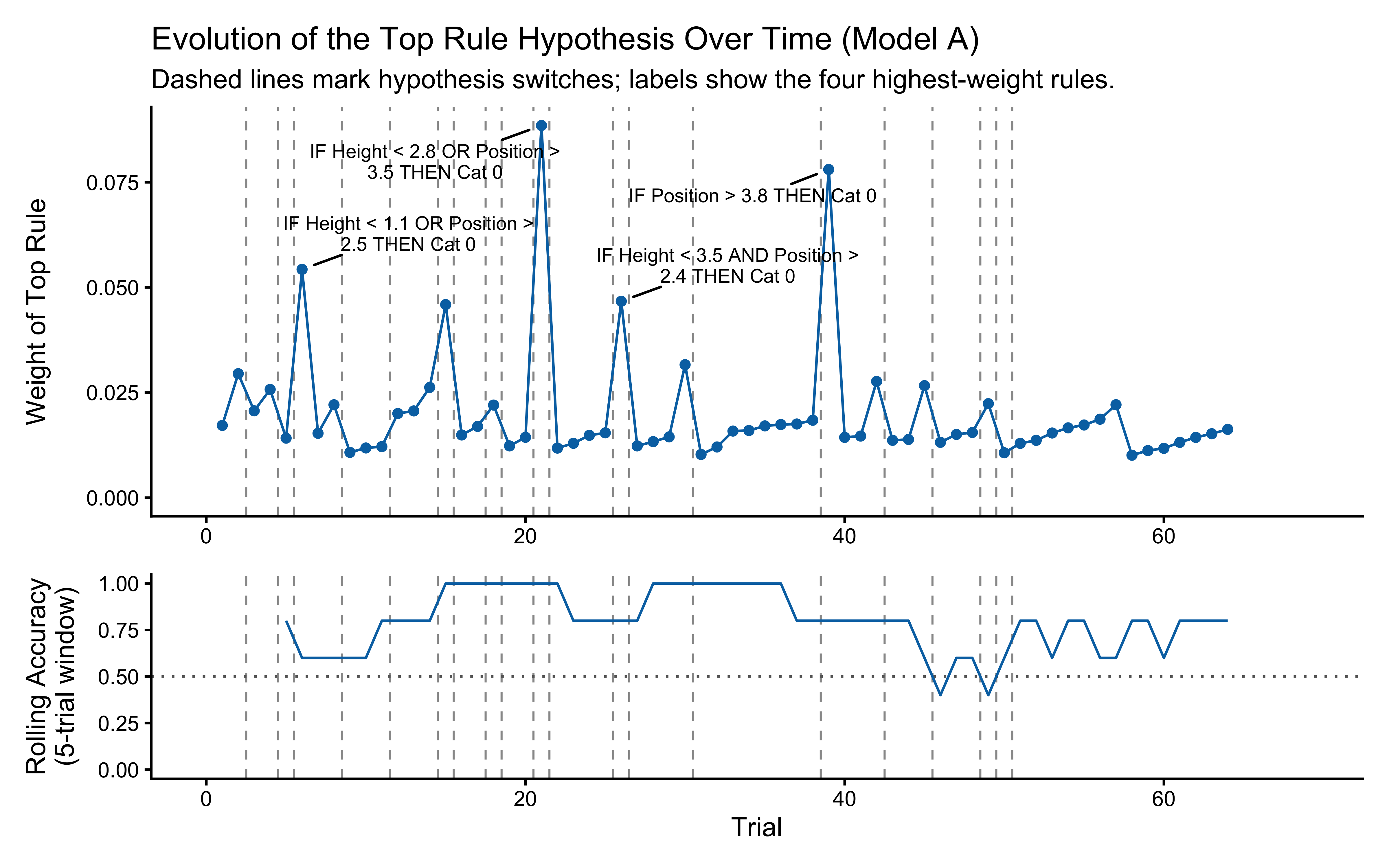
**Top panel — hypothesis weight.** The line tracks the probability assigned to whichever rule particle currently has the highest weight. Two features stand out. First, the weight never exceeds roughly 0.09: the filter never commits to a single rule, remaining diffuse across the full particle set throughout learning. Second, dashed vertical lines mark every moment the top-ranked rule changes identity — these switches are frequent, especially early on, as the filter resamples and mutates the particle population in response to prediction errors.
**Bottom panel — rolling accuracy.** The 5-trial rolling accuracy of the agent's actual responses (drawn from the full weighted ensemble) is shown on the same time axis, with a dotted reference line at chance (0.5). A key observation is that performance does *not* dip at every hypothesis switch. This is because the agent's response is determined by the collective vote of all particles, not by the top rule alone: many particles may agree on the correct prediction even while the highest-weight particle changes identity. Accuracy falls noticeably only when the ensemble as a whole is confused — not merely when one particle loses its rank. This dissociation between hypothesis instability and behavioural stability is a defining feature of particle-filter cognition.
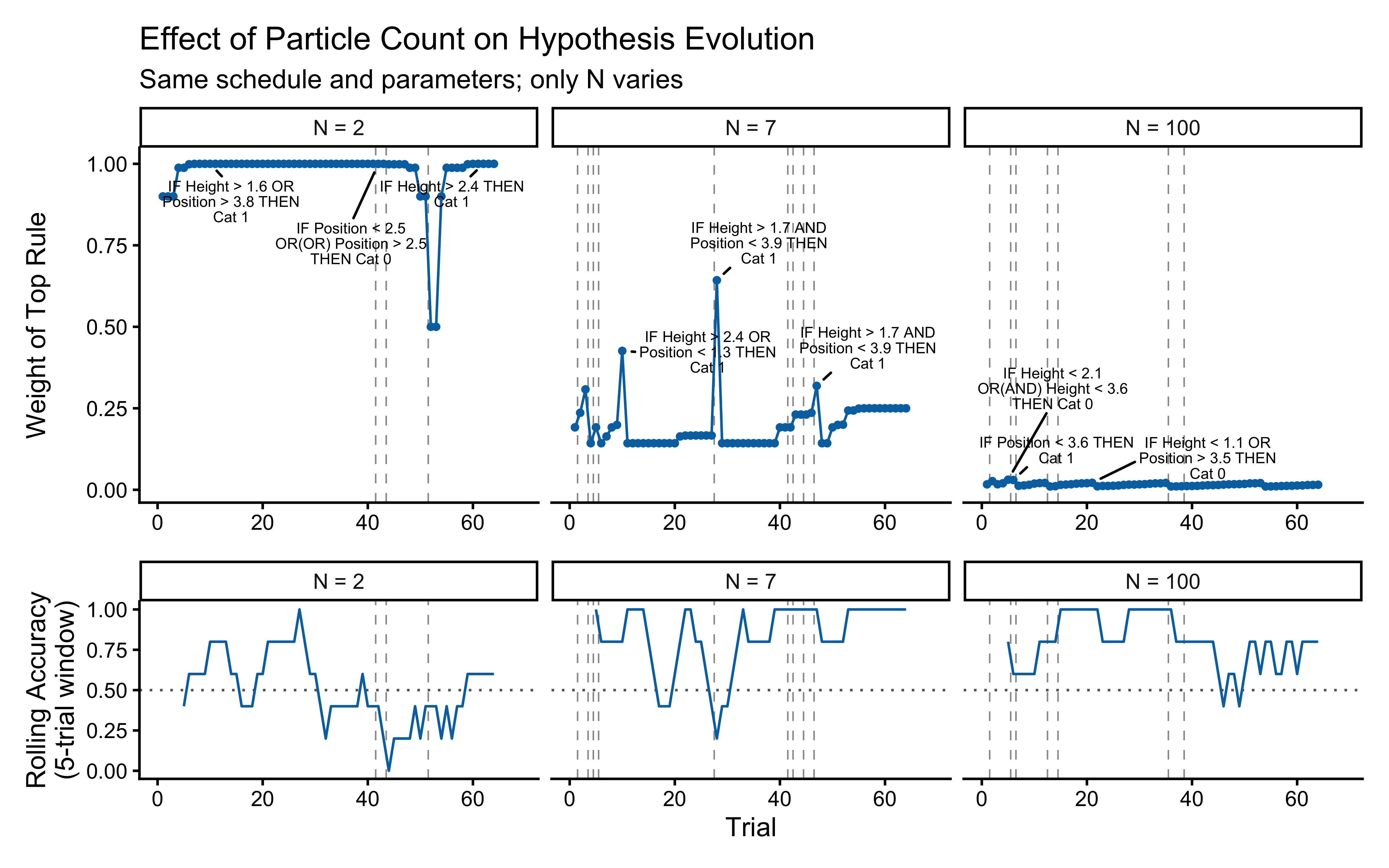
How much of this stability is due to ensemble size? The comparison below repeats the same schedule with $N = 2$, $N = 7$, and the default $N = `r N_PARTICLES_FIXED`$ particles.
```{r ch15_particle_count_comparison}
np_compare <- c(2L, 7L, N_PARTICLES_FIXED)

# Collect tracking and performance data for each particle count
compare_tracking <- map_dfr(np_compare, function(np) {
  set.seed(1)
  track_rule_learning(
    n_particles   = np,
    error_prob    = 0.1,
    mutation_prob = plogis(LOGIT_MU_PRIOR_MEAN),
    obs           = as.matrix(track_schedule[, c("height", "position")]),
    cat_one       = track_schedule$category_feedback,
    max_dims      = MAX_RULE_DIMS,
    top_k         = 1
  ) |> mutate(n_particles = np)
})

compare_plot_data <- compare_tracking |>
  filter(rank == 1) |>
  rowwise() |>
  mutate(rule_text = rule_to_text(cur_data())) |>
  ungroup() |>
  group_by(n_particles) |>
  mutate(rule_block = consecutive_id(rule_text)) |>
  ungroup()

compare_switches <- compare_plot_data |>
  group_by(n_particles, rule_block) |>
  summarise(switch_trial = min(trial), .groups = "drop") |>
  filter(switch_trial > 1)

compare_top_labels <- compare_plot_data |>
  group_by(n_particles, rule_block, rule_text) |>
  slice_max(weight, n = 1, with_ties = FALSE) |>
  ungroup() |>
  group_by(n_particles) |>
  slice_max(weight, n = 3) |>
  ungroup() |>
  mutate(rule_text = str_wrap(rule_text, width = 22))

compare_perf <- map_dfr(np_compare, function(np) {
  set.seed(1)
  tf <- rule_particle_filter(
    n_particles   = np,
    error_prob    = 0.1,
    mutation_prob = plogis(LOGIT_MU_PRIOR_MEAN),
    obs           = as.matrix(track_schedule[, c("height", "position")]),
    cat_one       = track_schedule$category_feedback,
    max_dims      = MAX_RULE_DIMS,
    quiet         = TRUE
  )
  tibble(
    trial       = seq_len(nrow(track_schedule)),
    correct     = as.integer(tf$sim_response == track_schedule$category_feedback),
    n_particles = np
  ) |>
    mutate(rolling_acc = slider::slide_dbl(correct, mean, .before = 4, .complete = TRUE))
})

np_labeller <- as_labeller(function(x) paste0("N = ", x))

p_compare_weights <- ggplot(compare_plot_data, aes(x = trial, y = weight)) +
  geom_vline(
    data = compare_switches, aes(xintercept = switch_trial - 0.5),
    linetype = "dashed", color = "grey60", linewidth = 0.3
  ) +
  geom_line(aes(group = 1), color = "#0072B2") +
  geom_point(color = "#0072B2", size = 1) +
  geom_text_repel(
    data = compare_top_labels, aes(label = rule_text),
    size = 2.2, lineheight = 0.85,
    box.padding = 0.4, point.padding = 0.2,
    max.overlaps = Inf, min.segment.length = 0
  ) +
  facet_wrap(~n_particles, nrow = 1, labeller = np_labeller) +
  scale_x_continuous(limits = c(0, total_trials + 5)) +
  scale_y_continuous(name = "Weight of Top Rule") +
  labs(
    title    = "Effect of Particle Count on Hypothesis Evolution",
    subtitle = "Same schedule and parameters; only N varies",
    x = NULL
  )

p_compare_perf <- ggplot(compare_perf, aes(x = trial, y = rolling_acc)) +
  geom_vline(
    data = compare_switches, aes(xintercept = switch_trial - 0.5),
    linetype = "dashed", color = "grey60", linewidth = 0.3
  ) +
  geom_hline(yintercept = 0.5, linetype = "dotted", color = "grey40") +
  geom_line(color = "#0072B2") +
  facet_wrap(~n_particles, nrow = 1, labeller = np_labeller) +
  scale_x_continuous(limits = c(0, total_trials + 5)) +
  scale_y_continuous(limits = c(0, 1), name = "Rolling Accuracy\n(5-trial window)") +
  labs(x = "Trial")

p_compare_weights / p_compare_perf + plot_layout(heights = c(2, 1))
```
With $N = 2$ the filter holds only two competing rules at any moment: weights are near 0.5 each, one rule dominates for a stretch then abruptly gives way, and performance swings widely because a single bad particle can drag the ensemble vote. With $N = 7$ switching is still frequent but the top-rule weight is lower (probability is spread across more alternatives) and performance is somewhat smoother. With $N = `r N_PARTICLES_FIXED`$ the ensemble vote is stable enough that hypothesis instability in the top rule has little effect on accuracy. This illustrates why $N$ carries cognitive content: it controls the trade-off between the precision of hypothesis tracking and the robustness of behavioural output.
### Visualizing the Decision Boundary
Rule-based models typically create axis-aligned, rectangular decision boundaries. Let's visualize the boundary created by the final, most probable rule found by Model A.
```{r ch15_decision_boundary}
get_final_rule_predictions <- function(n_particles, error_prob,
                                       obs_train, cat_one_train,
                                       grid_points, max_dims = MAX_RULE_DIMS,
                                       resample_threshold_factor = RESAMPLE_THRESHOLD) {
  n_features <- ncol(obs_train)
  fr         <- lapply(seq_len(n_features), function(d) range(obs_train[, d]))

  ps        <- initialize_particles(n_particles, n_features, max_dims, fr)
  particles <- ps$particles
  weights   <- ps$weights

  for (i in seq_len(nrow(obs_train))) {
    stim    <- as.numeric(obs_train[i, ])
    weights <- update_weights(particles, weights, stim, cat_one_train[i], error_prob)
    ess     <- 1 / sum(weights^2)
    if (ess < n_particles * resample_threshold_factor) {
      rs        <- resample_particles(particles, weights)
      particles <- rs$particles
      weights   <- rs$weights
    }
  }

  apply(as.matrix(grid_points), 1, function(pt) {
    preds <- sapply(particles, evaluate_rule, stimulus = pt)
    sum(weights * ifelse(preds == 1, 1 - error_prob, error_prob))
  })
}

grid_pts <- expand.grid(
  height   = seq(min(stimulus_info$height)   - 0.5,
                 max(stimulus_info$height)   + 0.5, length.out = 50),
  position = seq(min(stimulus_info$position) - 0.5,
                 max(stimulus_info$position) + 0.5, length.out = 50)
)

# Use the same track_schedule for boundary visualization
boundary_preds <- get_final_rule_predictions(
  n_particles   = 200,
  error_prob    = 0.1,
  obs_train     = as.matrix(track_schedule[, c("height", "position")]),
  cat_one_train = track_schedule$category_feedback,
  grid_points   = grid_pts[, c("height", "position")],
  max_dims      = MAX_RULE_DIMS
)

grid_decision_data <- grid_pts |>
  mutate(
    rule_prob_cat1 = boundary_preds,
    rule_decision  = as.integer(rule_prob_cat1 > 0.5)
  )

ggplot() +
  geom_tile(data = grid_decision_data,
            aes(x = position, y = height, fill = factor(rule_decision)),
            alpha = 0.4) +
  stat_contour(data = grid_decision_data,
               aes(x = position, y = height, z = rule_prob_cat1),
               breaks = 0.5, color = "black", linewidth = 0.8) +
  geom_point(data = stimulus_info,
             aes(x = position, y = height,
                 color = factor(category_true), shape = factor(category_true)),
             size = 3) +
  scale_fill_manual(values  = c("0" = "#E69F00", "1" = "#56B4E9"),
                    name    = "Predicted Cat") +
  scale_color_manual(values = c("0" = "#0072B2", "1" = "#D55E00"),
                     name    = "True Category") +
  scale_shape_manual(values = c("0" = 16, "1" = 17), name = "True Category") +
  labs(
    title    = "Rule-Based Model Decision Boundary (Model A, Particle Filter)",
    subtitle = "Weighted average of final particle set (N=200, error=0.1)",
    x = "Position Feature", y = "Height Feature"
  ) +
  coord_cartesian(
    xlim = range(grid_decision_data$position),
    ylim = range(grid_decision_data$height)
  )
```
**Boundary Interpretation**: The background color shows the predicted category for each point in the feature space, based on the weighted vote of the final rule particles. The black contour marks the 50% threshold. Notice the characteristic axis-aligned, rectangular character of the boundary regions — a direct consequence of the threshold-based rule structure — in contrast to the smooth, curved boundaries that would emerge from similarity-based models.
::: {.callout-tip title="Beyond Selection: Enhancing the Particle Filter for Rule Discovery"}
The Bayesian particle filter, as implemented above, provides a powerful framework for modeling how learners evaluate competing rule hypotheses. By maintaining a weighted set of particles and using resampling, it efficiently focuses on rules that best explain observed data.
However, a critical point: the basic filter primarily acts as a **rule selection** mechanism rather than a **rule generation** engine. It excels at identifying the most promising rules from an *initially provided set*. If the truly optimal rule is complex or unusual and not present in the initial random pool, the basic resampling step (which only duplicates existing rules) cannot discover it.
To create a model that more actively explores and discovers better rules during learning, the basic particle filter can be augmented with additional mechanisms:
1. **Mutation/Perturbation**: Introduce small, random variations to rules after resampling — slightly adjust a threshold, flip a comparison operator, or change the dimension used in a condition. This allows fine-tuning and local exploration around currently successful rules.
2. **Recombination/Crossover**: Combine elements from two successful "parent" rules to create new "child" rules — for example, the first condition of Parent A with the second condition of Parent B. This allows synthesizing features discovered independently by different rules.
3. **Targeted Rule Generation**: Generate new rules specifically designed to address stimuli consistently misclassified by the current particle set, or focus on features prevalent in high-weight rules.
4. **Complexity Adjustment**: Probabilistically add a condition to a successful 1D rule to explore whether a 2D rule performs better, or simplify a poorly performing 2D rule into its constituent 1D components.
Incorporating such exploration mechanisms transforms the particle filter from a pure selection device into a more adaptive **rule discovery system** capable of generating and testing rules that were not part of the initial random set. We do not implement these extensions here, but they represent a natural direction for more cognitively realistic models of rule learning. Note also that any of these mechanisms makes Model A's intractability *worse*, not better, from an HMC standpoint — they all add stochastic discrete jumps. NPE handles them transparently: the inference network only sees simulated $(\theta, y)$ pairs and does not care how the simulator produces them.
:::
## Prior Predictive Check (Model A Simulator, Model B Prior)
Before fitting Model B we want to verify that the prior on `logit_error_prob` generates only scientifically plausible categorisation curves. There is a subtle issue: **the Stan model does not have a forward simulator with learning dynamics.** Model B is conditionally i.i.d. in $\varepsilon$, so its forward simulation is just "draw $\varepsilon$, draw a rule, generate Bernoulli responses." This produces flat learning curves at level $1 - \varepsilon$, which is empirically nothing like what the data look like.
What earlier drafts of this chapter did — and what we keep here, but flag explicitly — is to draw $\varepsilon$ from the Stan prior and then use **Model A's simulator** to generate the prior predictive learning curves. This is *not* a prior predictive check for Model B in the strict sense. It is a prior predictive check for the cognitive theory under Model B's $\varepsilon$ prior. The two are not the same and the reader should know which is being shown.
```{r ch15_prior_predictive_check}
n_ppc_samples <- 500
set.seed(42)

ppc_logit_eps <- rnorm(n_ppc_samples, LOGIT_ERROR_PRIOR_MEAN, LOGIT_ERROR_PRIOR_SD)
ppc_eps       <- plogis(ppc_logit_eps)
ppc_sched     <- make_subject_schedule(stimulus_info, n_blocks, seed = 999)

ppc_file <- here("simdata", "ch15_prior_pred_curves.csv")

if (regenerate_simulations || !file.exists(ppc_file)) {
  cat("Running prior predictive simulations...\n")
  prior_pred_curves <- future_map_dfr(seq_len(n_ppc_samples), function(s) {
    sim <- rule_particle_filter(
      n_particles = N_PARTICLES_FIXED,
      error_prob  = ppc_eps[s],
      obs         = as.matrix(ppc_sched[, c("height", "position")]),
      cat_one     = ppc_sched$category_feedback,
      max_dims    = MAX_RULE_DIMS,
      quiet       = TRUE
    )
    tibble(
      sample_id = s,
      trial     = seq_len(nrow(ppc_sched)),
      correct   = as.integer(sim$sim_response == ppc_sched$category_feedback)
    ) |>
      mutate(cum_acc = cumsum(correct) / row_number())
  }, .options = furrr_options(seed = TRUE))
  write_csv(prior_pred_curves, ppc_file)
} else {
  prior_pred_curves <- read_csv(ppc_file, show_col_types = FALSE)
}

ppc_summary <- prior_pred_curves |>
  group_by(trial) |>
  summarise(
    q05 = quantile(cum_acc, 0.05), q25 = quantile(cum_acc, 0.25),
    q50 = median(cum_acc),
    q75 = quantile(cum_acc, 0.75), q95 = quantile(cum_acc, 0.95),
    .groups = "drop"
  )

ggplot(ppc_summary, aes(x = trial)) +
  geom_ribbon(aes(ymin = q05, ymax = q95), fill = "#E69F00", alpha = 0.20) +
  geom_ribbon(aes(ymin = q25, ymax = q75), fill = "#E69F00", alpha = 0.40) +
  geom_line(aes(y = q50), color = "#B07D00", linewidth = 1) +
  geom_hline(yintercept = 0.5, linetype = "dashed", color = "grey40") +
  scale_y_continuous(limits = c(0, 1)) +
  labs(
    title    = "Prior Predictive Curves Under Model A's Simulator With Model B's ε Prior",
    subtitle = "WARNING: This is NOT a prior predictive check for Model B in the strict sense.\nModel B has no learning dynamics; its true forward sim would be flat at 1 - ε.",
    x = "Trial", y = "Cumulative Accuracy"
  )
```
> **⚠️ Cross-model warning explicit.** The plot above shows prior predictive learning curves drawn from the *particle filter* (Model A) using $\varepsilon$ values sampled from the Stan model's (Model B's) prior. The Stan model fitted to the same data assumes no learning, so its true prior predictive distribution would consist of flat curves at $1 - \varepsilon$ — nothing like the rising curves shown here. We display these curves anyway because they are the most informative thing to show pedagogically (they convey the range of behaviour the cognitive theory produces under Model B's $\varepsilon$ prior), but they are a *cross-model* prior predictive, not a pure within-model one. The reader who wants the strict within-model check should compute it as: for each sample $s$, draw $\varepsilon_s$, draw a rule index $r_s \in \{1, \ldots, 5\}$ uniformly, and generate Bernoulli responses with probability $\Pr(\text{cat 1} \mid x_i, r_s, \varepsilon_s)$. The result is flat. It is also not very interesting.
---
## Model B: A Tractable Stan Proxy via Marginalised Mixture
We now switch models. Everything in this section implements **Model B** — the static, conditionally exchangeable mixture over a fixed candidate rule set. Model B is **not** the same as Model A with a clever trick. It is a different generative process that admits HMC inference and the full validation pipeline. Validation of Model B tells us about Model B; it does not tell us about Model A. We will return to this distinction at every opportunity.
### Why a separate proxy model?
Model A cannot be fitted with HMC for the reasons in §"Why Model A's Likelihood is Intractable for HMC." The validation pipeline used throughout this book is designed around HMC and a tractable likelihood, and the model comparison framework in Chapter 15 needs ELPD scores that come from a proper Bayesian fit. Two responses:
1. **Build a tractable proxy in Stan and validate it under the standard pipeline.** This is what Model B does. The proxy is honest about being a proxy: it is not the cognitive theory, and its validation does not transfer.
2. **Fit Model A directly via simulator-based inference.** This is what NPE does. We do this in §"Neural Posterior Estimation for Model A." The chapter then compares the two posteriors as its main empirical contribution.
This subsection builds Model B. The NPE subsection comes later because pedagogically it makes sense to first see what the tractable proxy can and cannot do.
### Model B's Generative Structure
Model B enumerates a fixed set of candidate rules and marginalises over them analytically. This is identical in structure to the finite mixture models of Chapter 8, where discrete latent variables (mixture components) were summed out before any Stan code was written. Here the discrete latent variable is "which rule from the candidate set the agent follows." The marginalised likelihood for trial $i$ is:
$$p(y_i \mid x_i, \varepsilon) = \sum_{r=1}^{R} p(\text{rule} = r) \cdot p(y_i \mid x_i, \text{rule}_r, \varepsilon)$$
with a uniform prior over rules $p(\text{rule} = r) = 1/R$, implemented with `log_sum_exp` in Stan. Only the single continuous parameter $\varepsilon$ needs to be sampled.
We parameterise $\varepsilon$ on the logit scale — $\text{logit}(\varepsilon) \sim \text{Normal}(-2, 1)$ — which is unconstrained, avoids the boundary artefacts that afflict bounded parameters in HMC, and places prior mass primarily on low error rates (prior median $\varepsilon \approx 0.12$). This is the same parameterisation philosophy as `log_c` in Chapter 12.
**Critical structural facts about Model B that distinguish it from Model A:**
* **No learning dynamics.** Model B treats all trials as conditionally exchangeable given $\varepsilon$. There is no trial-by-trial weight update, no resampling, no rule discovery. The agent's behaviour is determined entirely by which rule it follows (drawn once from the candidate set) and the noise rate $\varepsilon$.
* **Fixed candidate rule set.** The $R = 7$ rules are picked by inspecting the Kruschke stimulus layout (5 flat rules + 2 nested rules of the form $A \text{ op } (B \text{ inner } C)$). This is a post-hoc choice; §"Discharging the Post-Hoc Rule Selection" tests sensitivity.
* **Closed-form Bernoulli likelihood.** Marginalised analytically with `log_sum_exp`. HMC handles it cleanly.
* **No path-dependence.** Standard PSIS-LOO is technically valid (see §"LFO-CV Does Not Apply Here").
```{tikz ch15_model_b_dag, echo=FALSE, fig.cap="Generative structure of Model B (Stan proxy). Left: standard plate notation. Right: Kruschke-style notation. The sole continuous parameter is $\\varepsilon$ (error probability), inferred with HMC. The discrete latent variable $r$ (which candidate rule the agent follows) is summed out analytically via \\texttt{log\\_sum\\_exp} before Stan sees the likelihood — hence the dashed node. There is no trial-to-trial dependency: all observations are conditionally i.i.d. given $\\varepsilon$.", fig.ext='png', fig.width=12, cache=TRUE}
\usetikzlibrary{positioning, shapes.geometric, arrows.meta, fit, backgrounds, calc}
\tikzset{
stochastic/.style={->, >={Latex[length=3mm]}, thick},
deterministic/.style={->, >={Latex[length=3mm]}, thick, dashed, draw=gray!70},
plate/.style={draw=black, thick, rounded corners, inner sep=10pt},
continuous/.style={circle, draw=black, thick, minimum size=1.2cm, inner sep=0pt},
discrete/.style={rectangle, draw=black, thick, minimum size=1.2cm},
observed/.style={fill=gray!30},
latent/.style={fill=white},
marginalized/.style={rectangle, draw=black, thick, minimum size=1.2cm, dashed},
pics/norm_dist/.style={code={
\draw[thin, gray] (-1.2,0) -- (1.2,0);
\draw[thick, blue] plot[domain=-1.2:1.2, samples=50] (\x, {0.8*exp(-3*\x*\x)});
\node[font=\footnotesize, below] at (0,0) {Normal};
}},
pics/uniform_dist/.style={code={
\draw[thin, gray] (-1.2,0) -- (1.2,0);
\draw[thick, blue] (-0.9,0.6) -- (0.9,0.6) -- (0.9,0) (-0.9,0) -- (-0.9,0.6);
\node[font=\footnotesize, below] at (0,0) {Uniform};
}},
pics/bern_dist/.style={code={
\draw[thin, gray] (-1,0) -- (1,0);
\draw[blue, line width=4pt] (-0.4, 0) -- (-0.4, 0.3);
\draw[blue, line width=4pt] (0.4, 0) -- (0.4, 0.8);
\node[font=\footnotesize, below] at (0,0) {Bernoulli};
}}
}
\begin{tikzpicture}
%% LEFT: STANDARD PLATE NOTATION
\node[font=\large\bfseries] at (0, 2.2) {Standard Plate Notation};
% Top-level parameters
\node[continuous, latent] (eps) at (0, 0) {$\varepsilon$};
% Rule — dashed rectangle = marginalized discrete latent
\node[marginalized, latent] (r) at (0, -2.5) {$r$};
\node[font=\small, below=0.05cm of r] {\textit{marginalized}};
% Observed
\node[continuous, observed] (x_t) at (-2, -5.5) {$x_t$};
\node[discrete, observed] (y_t) at ( 2, -5.5) {$y_t$};
\node[plate, fit=(x_t)(y_t), label={[anchor=south east, font=\small\bfseries]below right:$i=1\dots T$}] (pT) {};
% Arrows
\draw[stochastic] (eps) -- (r);
\draw[stochastic] (eps) -- (y_t);
\draw[deterministic] (r) -- (y_t);
\draw[deterministic] (x_t) -- (y_t);
%% RIGHT: KRUSCHKE-STYLE NOTATION
\node[font=\large\bfseries] at (11, 2.2) {Kruschke-Style Notation};
% Prior on epsilon
\coordinate (k_eps) at (11, 0); \draw (k_eps) pic {norm_dist};
\node[above=0.7cm of k_eps, font=\bfseries] {$\varepsilon$ (logit scale)};
% Rule prior (uniform, marginalized)
\coordinate (k_r) at (11, -2.5); \draw (k_r) pic {uniform_dist};
\node[above=0.7cm of k_r, font=\bfseries, align=center] {Rule $r \in \{1\dots R\}$};
\node[font=\small, below=1.0cm of k_r, align=center, text=gray] {\textit{summed out analytically}};
% Observed stimulus
\node[discrete, observed, minimum size=0.9cm] (k_x) at (8, -5.5) {$x_i$};
\node[above=0.5cm of k_x, font=\bfseries] {Stimulus};
% Response
\coordinate (k_y) at (14, -5.5); \draw (k_y) pic {bern_dist};
\node[above=0.9cm of k_y, font=\bfseries] {Response ($y_i$)};
% Trial plate
\draw[plate, dotted] (7.0, -7.0) rectangle (15.0, -4.5) node[below left, font=\small\bfseries] {$i=1\dots T$};
% Arrows
\draw[stochastic] (k_eps) -- (k_y) node[midway, right, font=\large]{$\sim$};
\draw[stochastic] (k_eps) -- (k_r);
\draw[deterministic] (k_r) -- (k_y);
\draw[deterministic] (k_x) -- (13.3, -5.5);
\end{tikzpicture}
```
### Stan Model
```{r ch15_stan_rule_model}
rule_simplified_stan <- "
// Model B: Marginalised Mixture over Fixed Candidate Rules
// This is NOT the cognitive theory (Model A, the particle filter).
// It is a tractable proxy that admits HMC validation.
// Validation of Model B tests Model B, not Model A.
//
// Architecture (identical in principle to Ch. 8 mixture models):
//   - Discrete latent variable = which rule the agent follows
//   - Marginalized analytically with log_sum_exp over a fixed rule set
//   - Only continuous parameter: logit_error_prob (unconstrained)
//   - error_prob = inv_logit(logit_error_prob)
//
// No sequential learning in this model: it treats all trials as conditionally
// exchangeable given error_prob and the rule mixture.
//
// The 7 rules below cover the main decision structures visible in the
// Kruschke stimulus layout, including two nested rules of the form
// A op (B inner C) that cannot be expressed as flat 2D conjunctions/disjunctions.
// See §'Discharging the Post-Hoc Rule Selection' for the sensitivity analysis.

data {
  int<lower=1> ntrials;
  int<lower=1> nfeatures;                       // must be 2 for this rule set
  array[ntrials] int<lower=0, upper=1> y;       // observed choices
  array[ntrials, nfeatures] real obs;           // obs[,1]=Height, obs[,2]=Position

  // Prior hyperparameters (passed as data for transparency)
  real prior_logit_error_mean;
  real<lower=0> prior_logit_error_sd;
}

parameters {
  real logit_error_prob;   // unconstrained; error_prob = inv_logit(logit_error_prob)
}

transformed parameters {
  real<lower=0, upper=1> error_prob = inv_logit(logit_error_prob);

  // Per-trial choice probability under each rule, computed once per leapfrog
  // step so log_lik in generated quantities is a one-line lookup.
  // (Same architectural discipline as Ch 11 GCM and Ch 12 prototype.)
  array[ntrials] real lp_marginal;

  for (i in 1:ntrials) {
    real h = obs[i, 1];
    real p = obs[i, 2];

    // -- Flat 1D and 2D rules (same as original 5) --------------------------
    int pred1 = h > 2.5 ? 1 : 0;
    int pred2 = p < 2.5 ? 1 : 0;
    int pred3 = (h > 2.0 && p > 3.0) ? 1 : 0;
    int pred4 = (h < 2.0 || p < 2.0) ? 0 : 1;
    int pred5 = (h > 2.5 && p < 3.5) ? 1 : 0;
    // -- Nested rules: A op (B inner C) -------------------------------------
    // pred6: (h > 3.5) OR ((h > 1.5) AND (p < 1.5))
    // Cognitive reading: very tall OR some height AND very low position
    // Perfectly classifies the 8 Kruschke stimuli.
    int pred6 = (h > 3.5 || (h > 1.5 && p < 1.5)) ? 1 : 0;
    // pred7: (h > 1.5) AND ((p < 2.5) OR (h > 3.5))
    // Cognitive reading: some height AND low position OR very tall
    // Also perfectly classifies the 8 Kruschke stimuli.
    int pred7 = (h > 1.5 && (p < 2.5 || h > 3.5)) ? 1 : 0;

    int R = 7;

    vector[R] lp;
    lp[1] = bernoulli_lpmf(y[i] | pred1 == 1 ? 1 - error_prob : error_prob);
    lp[2] = bernoulli_lpmf(y[i] | pred2 == 1 ? 1 - error_prob : error_prob);
    lp[3] = bernoulli_lpmf(y[i] | pred3 == 1 ? 1 - error_prob : error_prob);
    lp[4] = bernoulli_lpmf(y[i] | pred4 == 1 ? 1 - error_prob : error_prob);
    lp[5] = bernoulli_lpmf(y[i] | pred5 == 1 ? 1 - error_prob : error_prob);
    lp[6] = bernoulli_lpmf(y[i] | pred6 == 1 ? 1 - error_prob : error_prob);
    lp[7] = bernoulli_lpmf(y[i] | pred7 == 1 ? 1 - error_prob : error_prob);

    lp_marginal[i] = log_sum_exp(lp) - log(R);
  }
}

model {
  target += normal_lpdf(logit_error_prob | prior_logit_error_mean, prior_logit_error_sd);
  for (i in 1:ntrials) target += lp_marginal[i];
}

generated quantities {
  // log_lik[i] is just a lookup of lp_marginal[i] -- no recomputation.
  array[ntrials] real log_lik;
  for (i in 1:ntrials) log_lik[i] = lp_marginal[i];

  real lprior = normal_lpdf(logit_error_prob | prior_logit_error_mean, prior_logit_error_sd);
}
"

stan_file_rule <- here("stan", "ch14_rule_simplified.stan")
write_stan_file(rule_simplified_stan, dir = "stan/",
                basename = "ch14_rule_simplified.stan")
mod_rule_stan <- cmdstan_model(stan_file_rule)
cat("Model B (Stan rule mixture) compiled successfully.\n")
```
**Key aspects of the Model B Stan implementation:**
* **Parameters block**: A single scalar `logit_error_prob` (unconstrained). The constraint `error_prob ∈ (0,1)` is enforced implicitly by `inv_logit`.
* **Transformed parameters**: The marginalised log-density per trial (`lp_marginal[i]`) is computed once per leapfrog step. This is the same `transformed parameters` discipline as Chapter 12 (GCM) and Chapter 13 (Kalman prototype): if a quantity depends on parameters but is otherwise deterministic given the data, it belongs in `transformed parameters` so generated quantities can read it without recomputation.
* **Model block**: Prior on `logit_error_prob` then accumulation of `lp_marginal[i]` into the target.
* **Generated quantities**: `log_lik[i]` is a one-line lookup. Architecturally consistent with the other two chapters.
### Fitting Model B
```{r ch15_fit_stan_rule_model}
# Simulate responses from one Model A agent to use as 'observed' data
fit_schedule <- make_subject_schedule(stimulus_info, n_blocks, seed = 42)
fit_sim <- rule_particle_filter(
  n_particles = N_PARTICLES_FIXED,
  error_prob  = 0.1,
  obs         = as.matrix(fit_schedule[, c("height", "position")]),
  cat_one     = fit_schedule$category_feedback,
  max_dims    = MAX_RULE_DIMS,
  quiet       = TRUE
)

rule_data_single <- list(
  ntrials                 = nrow(fit_schedule),
  nfeatures               = 2L,
  y                       = as.integer(fit_sim$sim_response),
  obs                     = as.matrix(fit_schedule[, c("height", "position")]),
  prior_logit_error_mean  = LOGIT_ERROR_PRIOR_MEAN,
  prior_logit_error_sd    = LOGIT_ERROR_PRIOR_SD
)

fit_filepath_rule <- here("simmodels", "ch14_rule_single_fit.rds")
if (regenerate_simulations || !file.exists(fit_filepath_rule)) {
  pf_rule <- mod_rule_stan$pathfinder(
    data      = rule_data_single,
    seed      = 42,
    num_paths = 4,
    refresh   = 0
  )

  fit_rule_stan <- mod_rule_stan$sample(
    data            = rule_data_single,
    init            = pf_rule,
    seed            = 42,
    chains          = 4,
    parallel_chains = min(4, availableCores()),
    iter_warmup     = 1000,
    iter_sampling   = 1500,
    refresh         = 300,
    adapt_delta     = 0.9
  )
  fit_rule_stan$save_object(fit_filepath_rule)
  cat("Model B fitted and saved.\n")
} else {
  if (file.exists(fit_filepath_rule)) {
    fit_rule_stan <- readRDS(fit_filepath_rule)
    cat("Loaded existing Model B fit.\n")
  } else {
    cat("Fit file not found. Set regenerate_simulations = TRUE.\n")
    fit_rule_stan <- NULL
  }
}
if (!is.null(fit_rule_stan)) {
  param_summary <- fit_rule_stan$summary(
    variables = c("logit_error_prob", "error_prob")
  )
  print(param_summary)
}
```
### Mandatory MCMC Diagnostic Battery
We need to curate the diagnostics, even when they are nearly trivial (see @sec-model-quality-checks). Use the same `diagnostic_summary_table()` helper as Chapters 11 and 12.
```{r ch15_diag_battery_model_B}
if (!is.null(fit_rule_stan)) {
  diag_tbl <- diagnostic_summary_table(
    fit_rule_stan,
    params = c("logit_error_prob", "error_prob")
  )
  print(diag_tbl)

  cat("\nThreshold reference (see @sec-model-quality-checks):\n",
      "  divergences        = 0\n",
      "  rank-normalized Rhat < 1.01\n",
      "  bulk ESS           > 400\n",
      "  tail ESS           > 400\n",
      "  E-BFMI             > 0.2\n",
      "  MCSE_mean / SD     < 0.05\n", sep = "")

  p_trace <- bayesplot::mcmc_trace(
    fit_rule_stan$draws(c("logit_error_prob", "error_prob")),
    facet_args = list(ncol = 2)
  ) +
    ggtitle("Trace plots — should look like hairy caterpillars")

  p_rank <- bayesplot::mcmc_rank_overlay(
    fit_rule_stan$draws(c("logit_error_prob", "error_prob")),
    facet_args = list(ncol = 2)
  ) +
    ggtitle("Rank histograms — should be uniform across chains")

  print(p_trace / p_rank)
}
```
### Posterior Predictive Check (Model B)
The posterior predictive check is honest about being a check on Model B, not on the cognitive theory. We sample $\varepsilon$ from the posterior, draw a rule index $r$ uniformly from the candidate set, and generate Bernoulli responses. The result is what Model B *actually* predicts: a flat-mean response sequence with whatever variation the rule mixture provides.
```{r ch15_ppc_model_B}
if (!is.null(fit_rule_stan)) {
  draws <- fit_rule_stan$draws("error_prob")
  eps_draws_df <- as_draws_df(draws)
  eps_draws  <- eps_draws_df$error_prob
  n_draws    <- length(eps_draws)
  obs_mat    <- as.matrix(fit_schedule[, c("height", "position")])
  R_rules    <- 7L
  n_obs      <- nrow(fit_schedule)

  # Per-rule predictions on the observed stimulus sequence (7 rules: 5 flat + 2 nested)
  rule_preds <- matrix(0L, nrow = R_rules, ncol = n_obs)
  for (i in seq_len(n_obs)) {
    h <- obs_mat[i, 1]; p <- obs_mat[i, 2]
    rule_preds[1, i] <- as.integer(h > 2.5)
    rule_preds[2, i] <- as.integer(p < 2.5)
    rule_preds[3, i] <- as.integer(h > 2.0 && p > 3.0)
    rule_preds[4, i] <- as.integer(!(h < 2.0 || p < 2.0))
    rule_preds[5, i] <- as.integer(h > 2.5 && p < 3.5)
    rule_preds[6, i] <- as.integer(h > 3.5 || (h > 1.5 && p < 1.5))  # nested: OR with inner AND
    rule_preds[7, i] <- as.integer(h > 1.5 && (p < 2.5 || h > 3.5))  # nested: AND with inner OR
  }

  set.seed(2026)
  yrep <- matrix(0L, nrow = n_draws, ncol = n_obs)
  for (s in seq_len(n_draws)) {
    r_idx     <- sample.int(R_rules, 1)
    rule_pred <- rule_preds[r_idx, ]
    p_cat1    <- ifelse(rule_pred == 1, 1 - eps_draws[s], eps_draws[s])
    yrep[s, ] <- rbinom(n_obs, 1, p_cat1)
  }

  # Cumulative-accuracy ribbons vs. observed
  obs_correct <- as.integer(fit_sim$sim_response == fit_schedule$category_feedback)
  obs_cum_acc <- cumsum(obs_correct) / seq_len(n_obs)
  yrep_correct <- sweep(yrep, 2,
                        as.numeric(fit_schedule$category_feedback),
                        FUN = function(a, b) as.numeric(a == b))
  yrep_correct <- matrix(yrep_correct, nrow = n_draws, ncol = n_obs)

  yrep_cum_acc <- t(apply(yrep_correct, 1, function(r) cumsum(r) / seq_along(r)))

  cum_acc_summary <- tibble(
    trial = seq_len(n_obs),
    q05   = apply(yrep_cum_acc, 2, quantile, 0.05),
    q25   = apply(yrep_cum_acc, 2, quantile, 0.25),
    q50   = apply(yrep_cum_acc, 2, quantile, 0.50),
    q75   = apply(yrep_cum_acc, 2, quantile, 0.75),
    q95   = apply(yrep_cum_acc, 2, quantile, 0.95),
    obs   = obs_cum_acc
  )

  ggplot(cum_acc_summary, aes(x = trial)) +
    geom_ribbon(aes(ymin = q05, ymax = q95), fill = "#56B4E9", alpha = 0.20) +
    geom_ribbon(aes(ymin = q25, ymax = q75), fill = "#56B4E9", alpha = 0.40) +
    geom_line(aes(y = q50), color = "#0072B2", linewidth = 1) +
    geom_line(aes(y = obs), color = "#D55E00", linewidth = 1) +
    geom_hline(yintercept = 0.5, linetype = "dashed", color = "grey50") +
    labs(
      title    = "Posterior Predictive Check (Model B)",
      subtitle = "Blue: Model B's posterior predictive\nOrange: observed (generated by Model A)\nThe gap is informative — Model B has no learning curve.",
      x = "Trial", y = "Cumulative accuracy"
    ) +
    coord_cartesian(ylim = c(0.4, 1))
}
```
**Reading this plot.** The blue ribbons are Model B's actual posterior predictive cumulative accuracy. They are **flat across trials**, because Model B has no learning dynamics. The orange line is the observed data, generated by Model A, which *does* have learning dynamics. **The systematic gap is the structural misspecification of Model B**, made visible. This is exactly what the chapter wants the reader to see: Model B can recover an $\varepsilon$ value that fits the *average* response, but it cannot reproduce the trial-by-trial structure because that structure comes from a process Model B does not have.
### Prior–Posterior Update Plot (Model B)
```{r ch15_prior_posterior_update}
if (!is.null(fit_rule_stan)) {
  draws_df <- as_draws_df(fit_rule_stan$draws(c("logit_error_prob", "error_prob")))

  set.seed(7)
  n_prior <- nrow(draws_df)
  prior_logit_eps <- rnorm(n_prior, LOGIT_ERROR_PRIOR_MEAN, LOGIT_ERROR_PRIOR_SD)
  prior_eps       <- plogis(prior_logit_eps)

  prior_post_df <- bind_rows(
    tibble(scale = "logit_error_prob (computational)",
           value = prior_logit_eps, source = "prior"),
    tibble(scale = "logit_error_prob (computational)",
           value = draws_df$logit_error_prob, source = "posterior"),
    tibble(scale = "error_prob (interpretable)",
           value = prior_eps, source = "prior"),
    tibble(scale = "error_prob (interpretable)",
           value = draws_df$error_prob, source = "posterior")
  )

  true_lines <- tibble(
    scale = c("logit_error_prob (computational)", "error_prob (interpretable)"),
    value = c(qlogis(0.1), 0.1)
  )

  ggplot(prior_post_df, aes(x = value, fill = source, color = source)) +
    geom_density(alpha = 0.4, linewidth = 0.6) +
    geom_vline(data = true_lines,
               aes(xintercept = value),
               color = "red", linetype = "dashed") +
    facet_wrap(~ scale, scales = "free") +
    scale_fill_manual(values = c(prior = "#999999", posterior = "#E69F00")) +
    scale_color_manual(values = c(prior = "#666666", posterior = "#B07D00")) +
    labs(
      title    = "Prior → Posterior Update for Model B",
      subtitle = "Red dashed line = Model A's true generating ε = 0.1\nGap between posterior centre and the dashed line is the structural-bias signature.",
      x = NULL, y = "Density"
    )
}
```
The posterior should be substantially narrower than the prior. The relationship of the posterior centre to the dashed red line (the true $\varepsilon$ used to generate the data) is the **structural bias signature**: if the dashed line falls in the bulk of the posterior, the proxy is approximately faithful for this data; if the dashed line is in the tail or outside the posterior, the proxy is biased and the size of the offset is informative about how badly the candidate rule set misses the converged rule.
### Randomised LOO-PIT (Model B)
The same calibration check we used in Chapters 11 and 12, applied to Model B.
```{r ch15_loo_pit_randomised}
if (!is.null(fit_rule_stan)) {
  log_lik_mat <- fit_rule_stan$draws("log_lik", format = "matrix")
  psis_obj    <- loo::psis(log_lik_mat, cores = 4)

  log_w <- loo::weights.importance_sampling(psis_obj,
                                             normalize = TRUE,
                                             log = TRUE)

  # Compute LOO predictive probability of cat 1 from Model B
  # For this we need per-trial p_cat1 under each posterior draw and rule.
  # Easiest: sample rule per draw, compute p_cat1 = (1 - eps if rule says 1 else eps),
  # then average using LOO weights.
  eps_draws_full <- as_draws_df(fit_rule_stan$draws("error_prob"))$error_prob
  n_draws_full   <- length(eps_draws_full)
  n_obs          <- nrow(fit_schedule)

  set.seed(11)
  rule_idx_per_draw <- sample.int(7L, n_draws_full, replace = TRUE)

  # Per (draw, trial) p_cat1
  p_draws <- matrix(0, nrow = n_draws_full, ncol = n_obs)
  for (s in seq_len(n_draws_full)) {
    r <- rule_idx_per_draw[s]
    pred_row <- rule_preds[r, ]
    p_draws[s, ] <- ifelse(pred_row == 1,
                            1 - eps_draws_full[s],
                            eps_draws_full[s])
  }

  loo_p_cat1 <- vapply(seq_len(n_obs), function(i) {
    sum(exp(log_w[, i]) * p_draws[, i])
  }, numeric(1))

  y_obs <- as.integer(fit_sim$sim_response)
  set.seed(2026)
  rloo_pit <- vapply(seq_along(y_obs), function(i) {
    p_i <- loo_p_cat1[i]
    if (y_obs[i] == 1) runif(1, 1 - p_i, 1) else runif(1, 0, 1 - p_i)
  }, numeric(1))

  ggplot(tibble(rloo_pit = rloo_pit), aes(x = rloo_pit)) +
    geom_histogram(aes(y = after_stat(density)), bins = 20,
                   fill = "#E69F00", color = "white") +
    geom_hline(yintercept = 1, linetype = "dashed", color = "red") +
    labs(
      title    = "Randomised LOO-PIT (Model B)",
      subtitle = "If Model B is calibrated for this data, the histogram should look uniform on [0, 1]",
      x = "Randomised PIT value", y = "Density"
    ) +
    coord_cartesian(ylim = c(0, 2.5))
}
```
A roughly uniform histogram says Model B is calibrated *for the proxy task* (predicting individual binary responses given the posterior over $\varepsilon$ and the rule mixture). It does *not* say Model B is calibrated as a model of the cognitive process — that would require the NPE pipeline to validate Model A directly.
### LOO with Pareto-k as a Misspecification Diagnostic
```{r ch15_loo_rule}
if (!is.null(fit_rule_stan)) {
  loo_rule <- loo::loo(log_lik_mat, cores = 4)
  print(loo_rule)
  plot(loo_rule, label_points = TRUE,
       main = "PSIS-LOO Pareto-k: Model B")
}
```
Unlike Chapters 11 and 12, here the LOO ELPD is **technically valid** (Model B is conditionally exchangeable — see next subsection). But the Pareto-$\hat{k}$ values are still informative as a *misspecification diagnostic*: when Model B is misspecified relative to the true generating process (Model A), $\hat{k}$ values are likely to be elevated on the trials where the proxy fails most badly. Plotting $\hat{k}$ against trial number and stimulus identity localises the misspecification.
```{r ch15_pareto_k_by_trial_and_stimulus}
if (!is.null(fit_rule_stan)) {
  k_values <- loo_rule$diagnostics$pareto_k
  k_df <- tibble(
    trial      = seq_along(k_values),
    k_hat      = k_values,
    stimulus   = fit_schedule$stimulus_id,
    height     = fit_schedule$height,
    position   = fit_schedule$position,
    true_cat   = fit_schedule$category_feedback,
    obs_y      = fit_sim$sim_response
  )

  p_trial <- ggplot(k_df, aes(x = trial, y = k_hat)) +
    geom_point(aes(color = factor(true_cat)), size = 1.5) +
    geom_hline(yintercept = c(0.5, 0.7, 1.0),
               linetype = c("dotted", "dashed", "solid"),
               color = "red", alpha = 0.6) +
    scale_color_manual(values = c("0" = "#0072B2", "1" = "#D55E00"),
                       name = "True cat") +
    labs(
      title    = "Pareto-k by trial",
      subtitle = "Red lines: 0.5 (monitor), 0.7 (problematic), 1.0 (failed)",
      x = "Trial", y = "Pareto k"
    )

  p_stim <- ggplot(k_df, aes(x = factor(stimulus), y = k_hat)) +
    geom_boxplot(fill = "#E69F00", alpha = 0.6) +
    geom_jitter(width = 0.15, alpha = 0.4, size = 1) +
    geom_hline(yintercept = 0.7, linetype = "dashed", color = "red") +
    labs(
      title    = "Pareto-k by stimulus identity",
      subtitle = "If a particular stimulus has consistently elevated k_hat,\nthat stimulus is where the rule set fails",
      x = "Stimulus ID", y = "Pareto k"
    )

  print(p_trial / p_stim)
}
```
**Reading the Pareto-k plots as a misspecification diagnostic.** If the high-$\hat{k}$ values cluster on the *boundary stimuli* of the Kruschke set — the ones whose true category cannot be determined by any single rule from the candidate set — that is direct evidence that the rule set is missing the relevant boundary structure. If the high-$\hat{k}$ values cluster at *late trials*, that is a signal that Model A's particle filter has converged to a rule the candidate set does not contain, and Model B is using $\varepsilon$ inflation to absorb the systematic late-trial errors. In both cases, the diagnostic does not just say "the model is wrong" — it says **where the model is wrong**, which is much more useful.
### LFO-CV Does Not Apply Here
> **A back-reference, not a caveat to repeat.** Chapters 11 and 12 implement LFO-CV via `psis_lfo_gcm()` and `psis_lfo_kalman()` because the GCM and the Kalman prototype are path-dependent: trial $t$'s likelihood depends on the entire history of trials $1, \ldots, t-1$ through the memory or filter state. **Model B has no such path-dependence.** All trials are conditionally independent given $\varepsilon$ and the rule mixture: leaving out trial $t$ does not affect the likelihood of any other trial. Standard PSIS-LOO is therefore *exactly correct* for Model B and the LFO-CV machinery is unnecessary. We say this once here so the reader does not encounter the same caveat for the third time after seeing it twice in the previous chapters.
>
> A subtler point: when Chapter 15 compares Model B against the GCM (Chapter 12) and the Kalman prototype (Chapter 13), the comparison should be reported under each model's *correct* validation tool — LFO-CV for the path-dependent ones, standard LOO for Model B. ELPD differences across these tools are not directly commensurable on a fine scale, but they are commensurable enough to detect large effects. The bigger concern in Chapter 15 is the cross-architecture mismatch (Model B isn't even fitting the cognitive theory), and that concern is what the NPE subsection below resolves.
### Prior Sensitivity Analysis
```{r ch15_prior_sensitivity}
if (!is.null(fit_rule_stan)) {
  # Get all log_lik variable names (log_lik[1], log_lik[2], ...)
  all_params <- fit_rule_stan$metadata()$model_params
  log_lik_vars <- all_params[grep("^log_lik", all_params)]

  # Compute sensitivity
  ps <- priorsense::powerscale_sensitivity(fit_rule_stan, variable = c("error_prob"), log_lik = log_lik_vars)
  print(ps)

  # Try plotting if log_lik can be found automatically by create_priorsense_data
  try(priorsense::powerscale_plot_dens(fit_rule_stan, variables = c("error_prob")))
}
```
`powerscale_sensitivity()` reports a sensitivity index $\psi$ for each parameter. **One important limitation:** it perturbs only the *explicit* prior on `logit_error_prob`. It cannot detect sensitivity to the *implicit* prior over the rule set, which is the much bigger source of structural bias for Model B. Low $\psi$ here means Model B is robust to the parametric prior on $\varepsilon$ — it does *not* mean Model B is robust to the choice of candidate rules. The next subsection addresses that.
---
## Parameter Recovery (Model B)
We test recovery systematically across the plausible range of `error_prob`, with multiple independent datasets per true value, each with its own randomized stimulus schedule. **Caveat upfront:** the data are generated by Model A, fitted by Model B. If Model A converges to a rule that is not in Model B's candidate set, recovery will be biased. This is the structural-bias signature again.
```{r ch15_parameter_recovery}
run_rule_recovery <- function(true_error_prob, iteration,
                              stimulus_info, n_blocks) {
  subject_seed <- iteration * 1000 + round(true_error_prob * 1000)
  sched        <- make_subject_schedule(stimulus_info, n_blocks, seed = subject_seed)

  sim <- rule_particle_filter(
    n_particles = N_PARTICLES_FIXED,
    error_prob  = true_error_prob,
    obs         = as.matrix(sched[, c("height", "position")]),
    cat_one     = sched$category_feedback,
    max_dims    = MAX_RULE_DIMS,
    quiet       = TRUE
  )

  stan_dat <- list(
    ntrials                = nrow(sched),
    nfeatures              = 2L,
    y                      = as.integer(sim$sim_response),
    obs                    = as.matrix(sched[, c("height", "position")]),
    prior_logit_error_mean = LOGIT_ERROR_PRIOR_MEAN,
    prior_logit_error_sd   = LOGIT_ERROR_PRIOR_SD
  )

  pf <- tryCatch(
    mod_rule_stan$pathfinder(data = stan_dat, num_paths = 4,
                              refresh = 0, seed = subject_seed),
    error = function(e) NULL
  )
  init_val <- if (!is.null(pf)) pf else 0.5

  fit <- tryCatch(
    mod_rule_stan$sample(
      data = stan_dat, init = init_val,
      seed = subject_seed, chains = 2, parallel_chains = 2,
      iter_warmup = 800, iter_sampling = 1000,
      refresh = 0, adapt_delta = 0.9
    ),
    error = function(e) { cat("Fit error:", e$message, "\n"); NULL }
  )
  if (is.null(fit)) return(NULL)

  draws_eps <- fit$draws("error_prob", format = "df")
  tibble(
    true_error_prob   = true_error_prob,
    iteration         = iteration,
    estimated_eps_mean = mean(draws_eps$error_prob),
    est_lower_95      = quantile(draws_eps$error_prob, 0.025),
    est_upper_95      = quantile(draws_eps$error_prob, 0.975),
    had_divergence    = any(fit$diagnostic_summary(quiet = TRUE)$num_divergent > 0)
  )
}

eps_values_to_test <- c(0.05, 0.1, 0.15, 0.2, 0.3)
n_recovery_iters   <- 5   # increase to 20–50 for publication-quality recovery

recovery_file_rule <- here("simdata", "ch14_rule_recovery_results.rds")
if (regenerate_simulations || !file.exists(recovery_file_rule)) {
  cat("Running parameter recovery for Model B...\n")
  recovery_plan <- expand_grid(
    true_error_prob = eps_values_to_test,
    iteration       = seq_len(n_recovery_iters)
  )
  rule_recovery_results <- future_pmap_dfr(
    list(true_error_prob = recovery_plan$true_error_prob,
         iteration       = recovery_plan$iteration),
    run_rule_recovery,
    stimulus_info = stimulus_info,
    n_blocks      = n_blocks,
    .options = furrr_options(seed = TRUE)
  )
  saveRDS(rule_recovery_results, recovery_file_rule)
  cat("Recovery complete and saved.\n")
} else {
  rule_recovery_results <- readRDS(recovery_file_rule)
  cat("Recovery results loaded.\n")
}
ggplot(rule_recovery_results,
       aes(x = true_error_prob, y = estimated_eps_mean)) +
  geom_abline(intercept = 0, slope = 1, linetype = "dashed", color = "grey50") +
  geom_errorbar(aes(ymin = est_lower_95, ymax = est_upper_95,
                    color = had_divergence),
                width = 0.005, alpha = 0.7) +
  geom_point(aes(color = had_divergence), size = 3) +
  scale_color_manual(values = c("FALSE" = "#0072B2", "TRUE" = "#D55E00"),
                     name = "Had divergence") +
  labs(
    title    = "Parameter Recovery: Model B (error_prob)",
    subtitle = paste0("Points: posterior mean; bars: 95% CrI; n=",
                      n_recovery_iters,
                      " datasets per true value.\n",
                      "Data generated by Model A; fitted by Model B."),
    x = "True error_prob", y = "Estimated error_prob"
  )
```
**Discussion of Recovery Results.** Recovery of `error_prob` depends on whether Model B's candidate rule set contains rules that match what Model A converges to on each replicate. When the converged rule is in the candidate set, recovery is good. When it is not, Model B compensates by inflating $\varepsilon$ to absorb the systematic misclassifications, and the posterior mean shifts up — the points drift above the diagonal. This drift is the *quantitative* version of the structural-bias warning.
---
## Discharging the Post-Hoc Rule Selection
Model B's candidate rules are picked by inspecting the stimulus layout, which makes them empirical rather than prior. We discharge this in two complementary ways.
### Option 1: Sensitivity to the Candidate Rule Set
We define three alternative candidate rule sets and refit Model B on the same data:
* **Set A** — the 7 hand-picked rules (the ones in the Stan code above: 5 flat + 2 nested).
* **Set B** — 5 rules generated *blind* by running Model A on a separately-simulated training dataset and taking its top-weighted rules at the end of training. The training data is generated with $\varepsilon = 0.1$ on a different schedule than the fitting data. This is the "honest" version of the candidate set.
* **Set C** — 5 rules deliberately chosen to be *bad* (rules that disagree with most stimuli), as a stress test.
```{r ch15_rule_set_sensitivity}
# Helper to build a Stan model from a list of (predictor function) rules
build_stan_with_rules <- function(rule_predictors, name_suffix) {
  R <- length(rule_predictors)
  rule_lines <- paste(
    sprintf("    int pred%d = %s;", seq_len(R), rule_predictors),
    collapse = "\n"
  )
  lp_lines_model <- paste(
    sprintf("    lp[%d] = bernoulli_lpmf(y[i] | pred%d == 1 ? 1 - error_prob : error_prob);",
            seq_len(R), seq_len(R)),
    collapse = "\n"
  )

  stan_code <- sprintf("
data {
  int<lower=1> ntrials;
  int<lower=1> nfeatures;
  array[ntrials] int<lower=0, upper=1> y;
  array[ntrials, nfeatures] real obs;
  real prior_logit_error_mean;
  real<lower=0> prior_logit_error_sd;
}
parameters { real logit_error_prob; }
transformed parameters {
  real<lower=0, upper=1> error_prob = inv_logit(logit_error_prob);
  array[ntrials] real lp_marginal;
  for (i in 1:ntrials) {
    real h = obs[i, 1];
    real p = obs[i, 2];
%s
    int R = %d;
    vector[R] lp;
%s
    lp_marginal[i] = log_sum_exp(lp) - log(R);
  }
}
model {
  target += normal_lpdf(logit_error_prob | prior_logit_error_mean, prior_logit_error_sd);
  for (i in 1:ntrials) target += lp_marginal[i];
}
generated quantities {
  array[ntrials] real log_lik;
  for (i in 1:ntrials) log_lik[i] = lp_marginal[i];
  real lprior = normal_lpdf(logit_error_prob | prior_logit_error_mean, prior_logit_error_sd);
}
", rule_lines, R, lp_lines_model)

  fname <- here("stan", sprintf("ch14_rule_%s.stan",  name_suffix))
  write_stan_file(stan_code, dir = "stan/",
                  basename = sprintf("ch14_rule_%s.stan", name_suffix))
  cmdstan_model(fname, force_recompile = TRUE)
}

# Set A: hand-picked rules — 5 flat + 2 nested (replicates Model B exactly)
rules_A <- c(
  "h > 2.5 ? 1 : 0",
  "p < 2.5 ? 1 : 0",
  "(h > 2.0 && p > 3.0) ? 1 : 0",
  "(h < 2.0 || p < 2.0) ? 0 : 1",
  "(h > 2.5 && p < 3.5) ? 1 : 0",
  "(h > 3.5 || (h > 1.5 && p < 1.5)) ? 1 : 0",
  "(h > 1.5 && (p < 2.5 || h > 3.5)) ? 1 : 0"
)

# Set B: blind rules from a fresh Model A run on a separate seed
get_blind_rules <- function(seed = 7) {
  blind_sched <- make_subject_schedule(stimulus_info, n_blocks, seed = 50000 + seed)
  obs_b   <- as.matrix(blind_sched[, c("height", "position")])
  cat_b   <- blind_sched$category_feedback
  res     <- track_rule_learning(
    n_particles = N_PARTICLES_FIXED, error_prob = 0.1,
    obs = obs_b, cat_one = cat_b, max_dims = MAX_RULE_DIMS, top_k = 5
  )
  # Take the top 5 distinct rules at the final trial
  final <- res |> filter(trial == max(trial)) |>
    distinct(dimension1, operation1, threshold1,
             dimension2, operation2, threshold2,
             logic, prediction, .keep_all = TRUE) |>
    head(5)

  pred_strings <- character(nrow(final))
  for (k in seq_len(nrow(final))) {
    r <- final[k, ]
    feat1 <- if (r$dimension1 == 1) "h" else "p"
    cond1 <- sprintf("%s %s %.2f", feat1, r$operation1, r$threshold1)
    if (is.na(r$dimension2)) {
      pred_strings[k] <- sprintf("(%s) ? %d : %d", cond1, r$prediction, 1 - r$prediction)
    } else {
      feat2 <- if (r$dimension2 == 1) "h" else "p"
      cond2 <- sprintf("%s %s %.2f", feat2, r$operation2, r$threshold2)
      logic_op <- if (r$logic == "AND") "&&" else "||"
      pred_strings[k] <- sprintf("(%s %s %s) ? %d : %d",
                                  cond1, logic_op, cond2,
                                  r$prediction, 1 - r$prediction)
    }
  }
  pred_strings
}

rules_B <- get_blind_rules(seed = 7)

# Set C: deliberately bad rules
rules_C <- c(
  "h > 4.5 ? 1 : 0",        # virtually never fires
  "p > 4.5 ? 1 : 0",        # virtually never fires
  "h < 0.5 ? 1 : 0",        # virtually never fires
  "(h > 0.5 && p > 0.5) ? 1 : 0",  # always fires
  "(h > 0.5 || p > 0.5) ? 1 : 0"   # always fires
)

# Compile and fit each
mod_A <- build_stan_with_rules(rules_A, "setA")
mod_B <- build_stan_with_rules(rules_B, "setB")
mod_C <- build_stan_with_rules(rules_C, "setC")

fit_with_rules <- function(model, label) {
  fit <- model$sample(
    data = rule_data_single, init = 0.5, seed = 7,
    chains = 2, parallel_chains = 2,
    iter_warmup = 800, iter_sampling = 1000, refresh = 0, adapt_delta = 0.9
  )
  draws <- as_draws_df(fit$draws("error_prob"))
  tibble(
    rule_set     = label,
    posterior_mean = mean(draws$error_prob),
    posterior_lo = quantile(draws$error_prob, 0.025),
    posterior_hi = quantile(draws$error_prob, 0.975),
    elpd_loo     = loo::loo(fit$draws("log_lik", format = "matrix"))$estimates["elpd_loo", "Estimate"]
  )
}

rule_set_sensitivity_file <- here("simdata", "ch14_rule_set_sensitivity.rds")
if (regenerate_simulations || !file.exists(rule_set_sensitivity_file)) {
  rule_set_results <- bind_rows(
    fit_with_rules(mod_A, "A: hand-picked"),
    fit_with_rules(mod_B, "B: blind from Model A"),
    fit_with_rules(mod_C, "C: deliberately bad")
  )
  saveRDS(rule_set_results, rule_set_sensitivity_file)
} else {
  rule_set_results <- readRDS(rule_set_sensitivity_file)
}

if (exists("rule_set_results")) {
  print(rule_set_results)

  ggplot(rule_set_results,
         aes(x = rule_set, y = posterior_mean)) +
    geom_pointrange(aes(ymin = posterior_lo, ymax = posterior_hi)) +
    geom_hline(yintercept = 0.1, linetype = "dashed", color = "red") +
    labs(
      title = "Sensitivity of Model B's ε posterior to candidate rule set",
      subtitle = "Red dashed: true ε = 0.1 used to generate the data",
      x = NULL, y = "Posterior mean ± 95% CrI for ε"
    ) +
    coord_flip()
}
```
**Reading the rule-set sensitivity.** If the three posteriors agree, the candidate-set choice is innocuous. If they disagree — which is the expected outcome — the gap quantifies how much of Model B's estimated $\varepsilon$ is *cognitive* (genuinely tracking the agent's error rate) vs *structural* (compensating for missing rules). Set C should produce a wildly inflated $\varepsilon$ and a much worse ELPD, providing the upper bound on how much rule-set choice can move the posterior.
### Sensitivity to `max_dims` (Rule Grammar Depth)
```{r ch15_max_dims_sensitivity}
max_dims_results_file <- here("simdata", "ch14_max_dims_sensitivity.rds")
if (regenerate_simulations || !file.exists(max_dims_results_file)) {
  cat("Sweeping max_dims...\n")
  max_dims_results <- map_dfr(c(1, 2, 3), function(md) {
    tryCatch({
      sched <- make_subject_schedule(stimulus_info, n_blocks, seed = 42)
      sim_md <- rule_particle_filter(
        n_particles = N_PARTICLES_FIXED,
        error_prob  = 0.1,
        obs         = as.matrix(sched[, c("height", "position")]),
        cat_one     = sched$category_feedback,
        max_dims    = md
      )
      cum_acc <- mean(sim_md$sim_response == sched$category_feedback)
      tibble(max_dims = md, mean_accuracy = cum_acc)
    }, error = function(e) {
      tibble(max_dims = md, mean_accuracy = NA_real_)
    })
  })
  saveRDS(max_dims_results, max_dims_results_file)
} else {
  max_dims_results <- readRDS(max_dims_results_file)
}

if (exists("max_dims_results")) {
  print(max_dims_results)
  cat("Note: max_dims = 3 will fall back to 2 in our 2-feature task.\n",
      "The point of this sweep is to make the structural choice visible,\n",
      "not to discover anything new.\n")
}
```
`max_dims` is a structural commitment of the rule grammar. In our 2-feature task it can be 1 or 2 (3 is meaningless). In a higher-dimensional task it would be a genuine free parameter and should be either fixed with explicit cognitive justification or inferred via NPE.
### Sensitivity to Resampling Threshold
The chapter fixes `RESAMPLE_THRESHOLD = 0.5`. This controls how aggressively the particle filter reorganises its hypothesis set: lower values allow more particle degeneracy before resampling; higher values trigger resampling earlier. The cognitive interpretation is something like "how quickly the learner abandons low-performing hypotheses."
```{r ch15_resample_threshold_sensitivity}
resample_sensitivity_file <- here("simdata", "ch14_resample_threshold_sensitivity.rds")
if (regenerate_simulations || !file.exists(resample_sensitivity_file)) {
  cat("Sweeping resampling threshold...\n")
  resample_results <- map_dfr(c(0.25, 0.50, 0.75), function(rt) {
    accs <- vapply(1:10, function(rep) {
      sched <- make_subject_schedule(stimulus_info, n_blocks, seed = 42000 + rep)
      sim <- rule_particle_filter(
        n_particles               = N_PARTICLES_FIXED,
        error_prob                = 0.1,
        obs                       = as.matrix(sched[, c("height", "position")]),
        cat_one                   = sched$category_feedback,
        max_dims                  = MAX_RULE_DIMS,
        resample_threshold_factor = rt,
        quiet                     = TRUE
      )
      mean(sim$sim_response == sched$category_feedback)
    }, numeric(1))
    tibble(resample_threshold = rt,
           mean_accuracy = mean(accs), sd_accuracy = sd(accs))
  })
  saveRDS(resample_results, resample_sensitivity_file)
} else {
  resample_results <- readRDS(resample_sensitivity_file)
}

if (exists("resample_results")) {
  print(resample_results)
  cat("If mean accuracy varies substantially across thresholds,\n",
      "the resampling threshold is a consequential structural choice.\n",
      "If it is roughly stable, the choice is innocuous for this task.\n")
}
```
### Option 2: Treat Set A as a Sensitivity Condition, Not a Canonical Model
Rather than use Set A as *the* Model B and add Set B as a "robustness check," the honest framing is to report all three sets as variants of Model B with no privileged status. The reader sees three posteriors instead of one and decides for themselves how much of the variation is structural. This is the framing we adopt for the chapter 15 model comparison, where Model B is reported as a *family* of proxies indexed by the candidate set rather than as a single point estimate.
---
## Calibration: Two Different Checks for Two Different Things
Earlier drafts of this chapter ran one block under the header "Simulation-Based Calibration (SBC)" that generated data with the particle filter (Model A) and fitted Model B. **That is not SBC.** Talts–Vehtari SBC requires the data to be drawn from the *same* generative model that is then fitted, so that the joint $(\theta, y)$ distribution of the inference model is what gets calibrated. When the generative and inferential models differ, what you are running is closer to a robustness check than a calibration check, and labelling it SBC is misleading.
We split the misnamed block into two correctly-labelled checks: (1) a **Cross-Model Calibration Check** (data from Model A, fitted by Model B) and (2) a **Real SBC for Model B** (data from Model B itself, fitted by Model B). The first is a robustness check; the second is the actual Talts–Vehtari calibration test.
### Cross-Model Calibration Check (NOT SBC)
**Procedure.** For each iteration $i = 1, \ldots, S$: draw $\varepsilon_i$ from the prior, simulate one dataset with Model A (the particle filter) using $\varepsilon_i$, fit Model B to that dataset, record the rank of $\varepsilon_i$ within Model B's posterior. Compute the rank ECDF.
**What a flat ECDF means here.** It means: under the specific misspecification of Model B for data from Model A, $\varepsilon$ happens to be recovered with the right *marginal* coverage. It does **not** mean Model B is calibrated in the Talts–Vehtari sense, because the joint $(\theta, y)$ distribution of the inference model is not the joint distribution of the data-generating process.
**Why we run it anyway.** Because it answers a useful practical question: "when I fit Model B to data that came from a richer generative process (Model A), are the resulting credible intervals approximately well-calibrated for the *cognitive* parameter $\varepsilon$?" The answer to that question is informative even though it is not what SBC is technically supposed to answer.
```{r ch15_cross_model_check}
if (run_intensive_checks) {
  n_cross_iters <- 500   # use >= 1000 for production

  cross_generator <- SBC_generator_function(
    function() {
      logit_eps_true <- rnorm(1, LOGIT_ERROR_PRIOR_MEAN, LOGIT_ERROR_PRIOR_SD)
      eps_true       <- plogis(logit_eps_true)

      sched <- make_subject_schedule(stimulus_info, n_blocks, seed = sample.int(1e8, 1))
      # NOTE: data drawn from Model A (the particle filter)
      sim <- rule_particle_filter(
        n_particles = N_PARTICLES_FIXED,
        error_prob  = eps_true,
        obs         = as.matrix(sched[, c("height", "position")]),
        cat_one     = sched$category_feedback,
        max_dims    = MAX_RULE_DIMS,
        quiet       = TRUE
      )

      list(
        variables = list(logit_error_prob = logit_eps_true),
        generated = list(
          ntrials                = nrow(sched),
          nfeatures              = 2L,
          y                      = as.integer(sim$sim_response),
          obs                    = as.matrix(sched[, c("height", "position")]),
          prior_logit_error_mean = LOGIT_ERROR_PRIOR_MEAN,
          prior_logit_error_sd   = LOGIT_ERROR_PRIOR_SD
        )
      )
    }
  )

  cross_backend <- SBC_backend_cmdstan_sample(
    mod_rule_stan,
    iter_warmup = 1000, iter_sampling = 1000,
    chains = 2, adapt_delta = 0.9, refresh = 0
  )

  cross_datasets <- generate_datasets(
    cross_generator,
    n_sims = n_cross_iters
  )

  cross_results <- compute_SBC(
    cross_datasets, cross_backend,
    cache_mode     = "results",
    cache_location = here("simdata", "ch14_cross_model_check_cache"),
    keep_fits      = FALSE
  )

  # Plotted as rank ECDF, but with explicit re-labelling in the title
  p1 <- plot_ecdf_diff(cross_results) +
    ggtitle("CROSS-MODEL CALIBRATION CHECK (not SBC)",
            subtitle = "Data: Model A. Fit: Model B. Flat ≠ calibrated, only marginally well-covered.")
  p2 <- plot_rank_hist(cross_results) +
    ggtitle("Cross-model rank histogram (not SBC)")
  print(p1 / p2)
}
```
**Reading this plot.** A flat curve here means Model B's $\varepsilon$ posterior covers Model A's true generating $\varepsilon$ at approximately the right marginal rate. This is *useful* — it tells you Model B is at least not catastrophically wrong as a tool for estimating cognitive error rates. But it does not say Model B's inference engine is calibrated in the Talts–Vehtari sense, because the data-generating distribution is not the inference model's joint distribution.
### Real SBC for Model B
For a proper Talts–Vehtari SBC of Model B, the generator must use Model B itself: draw $\varepsilon$ from the prior, draw a rule index from $\{1, \ldots, 5\}$ uniformly (mirroring Model B's mixture prior), and generate Bernoulli responses accordingly. Then fit Model B and check the rank distribution.
```{r ch15_real_sbc_model_B}
if (run_intensive_checks) {
  n_real_sbc_iters <- 500   # use >= 1000 for production

  real_sbc_generator <- SBC_generator_function(
    function() {
      logit_eps_true <- rnorm(1, LOGIT_ERROR_PRIOR_MEAN, LOGIT_ERROR_PRIOR_SD)
      eps_true       <- plogis(logit_eps_true)

      # Use the SAME generator as Model B's mixture: draw a rule, generate Bernoulli responses
      rule_idx <- sample.int(7L, 1)
      sched    <- make_subject_schedule(stimulus_info, n_blocks, seed = sample.int(1e8, 1))
      obs_mat  <- as.matrix(sched[, c("height", "position")])
      n_trials <- nrow(obs_mat)

      rule_pred_for_trial <- function(i) {
        h <- obs_mat[i, 1]; p <- obs_mat[i, 2]
        switch(rule_idx,
               as.integer(h > 2.5),
               as.integer(p < 2.5),
               as.integer(h > 2.0 && p > 3.0),
               as.integer(!(h < 2.0 || p < 2.0)),
               as.integer(h > 2.5 && p < 3.5),
               as.integer(h > 3.5 || (h > 1.5 && p < 1.5)),
               as.integer(h > 1.5 && (p < 2.5 || h > 3.5)))
      }
      preds  <- vapply(seq_len(n_trials), rule_pred_for_trial, integer(1))
      p_cat1 <- ifelse(preds == 1, 1 - eps_true, eps_true)
      y      <- rbinom(n_trials, 1, p_cat1)

      list(
        variables = list(logit_error_prob = logit_eps_true),
        generated = list(
          ntrials                = n_trials,
          nfeatures              = 2L,
          y                      = as.integer(y),
          obs                    = obs_mat,
          prior_logit_error_mean = LOGIT_ERROR_PRIOR_MEAN,
          prior_logit_error_sd   = LOGIT_ERROR_PRIOR_SD
        )
      )
    }
  )

  real_sbc_backend <- SBC_backend_cmdstan_sample(
    mod_rule_stan,
    iter_warmup = 1000, iter_sampling = 1000,
    chains = 2, adapt_delta = 0.9, refresh = 0
  )

  real_sbc_datasets <- generate_datasets(
    real_sbc_generator,
    n_sims = n_real_sbc_iters
  )

  real_sbc_results <- compute_SBC(
    real_sbc_datasets, real_sbc_backend,
    cache_mode     = "results",
    cache_location = here("simdata", "ch14_real_sbc_cache"),
    keep_fits      = FALSE
  )

  p1 <- plot_ecdf_diff(real_sbc_results) +
    ggtitle("REAL SBC for Model B (Talts–Vehtari)",
            subtitle = "Data: Model B's own mixture generator. Fit: Model B.")
  p2 <- plot_rank_hist(real_sbc_results) +
    ggtitle("Real SBC rank histogram for Model B")
  print(p1 / p2)
}
```
**Reading this plot.** This is the actual calibration check. A flat ECDF here means Stan correctly inverts Model B (Model B's inference engine is calibrated in the Talts–Vehtari sense). Systematic deviations would indicate a miscalibration in the Stan implementation itself — a sign error, an off-by-one in the marginalisation, or a prior-on-`logit_error_prob` mismatch. **This is the only diagnostic in the chapter that tests the Stan engine on its own terms.** The cross-model check above tests something else — it tests how Model B behaves when applied to data from a richer process — and that something else is informative but it is not SBC.
### Posterior SBC for Model B (Phase 6c)
We need to perform **Posterior SBC (PSBC)** (see @sec-model-quality-checks): instead of drawing true parameters from the prior, draw them from the *fitted posterior*. This tests calibration in the specific high-probability region the actual data force us into. A sampler can be globally unbiased (prior SBC passes) yet struggle locally (PSBC fails) or vice versa.
```{r ch15_psbc_model_B}
if (run_intensive_checks) {
  n_psbc_iters <- 500  # use >= 1000 for production

  if (!is.null(fit_rule_stan)) {
    # Draw true parameters from the fitted posterior, not the prior
    fitted_draws <- as_draws_df(fit_rule_stan$draws("logit_error_prob"))
    fitted_logit_eps <- fitted_draws$logit_error_prob

    psbc_generator <- SBC_generator_function(
      function() {
        # Draw from the POSTERIOR, not the prior
        logit_eps_true <- sample(fitted_logit_eps, 1)
        eps_true       <- plogis(logit_eps_true)

        # Generate from Model B's own mixture (same as real SBC; 7 rules)
        rule_idx <- sample.int(7L, 1)
        sched    <- make_subject_schedule(stimulus_info, n_blocks, seed = sample.int(1e8, 1))
        obs_mat  <- as.matrix(sched[, c("height", "position")])
        n_trials <- nrow(obs_mat)

        rule_pred_for_trial <- function(j) {
          h <- obs_mat[j, 1]; p <- obs_mat[j, 2]
          switch(rule_idx,
                 as.integer(h > 2.5),
                 as.integer(p < 2.5),
                 as.integer(h > 2.0 && p > 3.0),
                 as.integer(!(h < 2.0 || p < 2.0)),
                 as.integer(h > 2.5 && p < 3.5),
                 as.integer(h > 3.5 || (h > 1.5 && p < 1.5)),
                 as.integer(h > 1.5 && (p < 2.5 || h > 3.5)))
        }
        preds  <- vapply(seq_len(n_trials), rule_pred_for_trial, integer(1))
        p_cat1 <- ifelse(preds == 1, 1 - eps_true, eps_true)
        y      <- rbinom(n_trials, 1, p_cat1)

        list(
          variables = list(logit_error_prob = logit_eps_true),
          generated = list(
            ntrials                = n_trials,
            nfeatures              = 2L,
            y                      = as.integer(y),
            obs                    = obs_mat,
            prior_logit_error_mean = LOGIT_ERROR_PRIOR_MEAN,
            prior_logit_error_sd   = LOGIT_ERROR_PRIOR_SD
          )
        )
      }
    )

    psbc_backend <- SBC_backend_cmdstan_sample(
      mod_rule_stan,
      iter_warmup = 1000, iter_sampling = 1000,
      chains = 2, adapt_delta = 0.9, refresh = 0
    )

    psbc_datasets <- generate_datasets(
      psbc_generator,
      n_sims = n_psbc_iters
    )

    psbc_results <- compute_SBC(
      psbc_datasets, psbc_backend,
      cache_mode     = "results",
      cache_location = here("simdata", "ch14_psbc_cache"),
      keep_fits      = FALSE
    )

    p1 <- plot_ecdf_diff(psbc_results) +
      ggtitle("POSTERIOR SBC for Model B (Phase 6c)",
              subtitle = "True ε drawn from FITTED posterior, not the prior.\nTests local calibration in the high-probability region.")
    p2 <- plot_rank_hist(psbc_results) +
      ggtitle("Posterior SBC rank histogram for Model B")
    print(p1 / p2)
  }
}
```
**Reading this plot.** A flat ECDF here means Model B is calibrated *locally* around the posterior region that the actual data identified. If prior SBC passes but PSBC fails, the sampler is globally unbiased but locally struggles — a sign of geometry issues in the high-posterior region. If both pass, the Stan implementation is sound in both senses.
---
## Neural Posterior Estimation for Model A
Model A — the particle filter — has an **intractable likelihood**: there is no closed-form expression for $p(y \mid \theta)$. The resampling step introduces a sum over all possible particle trajectories that cannot be evaluated analytically, and the discrete rule space rules out the differentiable marginalisation tricks that Stan exploits. This is not unusual: many of the most cognitively realistic models in the literature share this property. Agent-based models, reinforcement-learning models with discrete latent states, and sequential Monte Carlo approximations all produce data through simulation but resist likelihood evaluation.
**Neural Posterior Estimation (NPE)** is the modern solution to this problem. The core idea is simple: instead of computing $p(y \mid \theta)$ directly, we train a neural network to approximate the posterior $p(\theta \mid y)$ from a large dataset of simulated $(\theta, y)$ pairs.
::: {.callout-note title="Comparison: HMC vs. NPE"}
The choice between Stan (HMC) and BayesFlow (NPE) is a trade-off between mathematical transparency and theoretical flexibility.
| Feature | Stan (HMC) | BayesFlow (NPE) |
|---|---|---|
| **Requirement** | Differentiable likelihood $p(y \mid \theta)$ | Forward simulator $y \sim p(y \mid \theta)$ |
| **Inference Cost** | High per subject (MCMC chains) | One-time training; near-zero per subject |
| **Validation** | SBC (Phase 6) | SBC + Expected Coverage (Phase 6) |
| **Flexibility** | Limited to tractable likelihoods | Fits any simulator (Model A) |
| **Diagnostic Signal** | Divergences, R-hat, ESS | Amortization gap, recovery scatter |
:::
### How NPE Works: The Four Steps
The method proceeds in four conceptual steps. Each step maps directly onto a code block below.
**Step 1 — Define a prior $p(\theta)$.** This plays the same role as in any Bayesian analysis. For Model A we have three parameters: $\varepsilon$ (error probability), $N_\text{particles}$ (working-memory capacity), and $\mu$ (mutation rate). We place weakly informative priors on each.
**Step 2 — Simulate a training dataset.** Draw a large number of parameter vectors $\theta^{(i)} \sim p(\theta)$, and for each one run the simulator to produce a synthetic response sequence $y^{(i)} \sim p(y \mid \theta^{(i)})$. The result is a dataset $\{(\theta^{(i)}, y^{(i)})\}_{i=1}^{N}$ of input-output pairs. This step is the main computational cost — it is done once and then "amortized."
**Step 3 — Train a conditional density estimator $q_\phi(\theta \mid y)$.** This is the neural network. Its job is to take a response sequence $y$ and output a probability distribution over $\theta$ — a full posterior distribution. The training objective is to minimize the Kullback–Leibler divergence between the approximate posterior and the true posterior:
$$\min_{\phi} \; \mathbb{E}_{p(\theta, y)}\!\left[-\log q_\phi(\theta \mid y)\right] \;\approx\; -\frac{1}{N}\sum_{i=1}^{N} \log q_\phi\!\left(\theta^{(i)} \mid y^{(i)}\right).$$
**Step 4 — Perform inference on the observed data.** Plug $y_\text{obs}$ into the trained network and sample $\theta \sim q_\phi(\theta \mid y_\text{obs})$. These samples are the approximate posterior — no additional simulation or MCMC warm-up required.
::: {.callout-tip title="Why the BayesFlow approach buys what it buys"}
Five design properties that motivate the architecture, restated from @radev2020amortized:
* **Asymptotic theoretical guarantees** for sampling from the true parameter posterior, given sufficient network capacity and training data.
* **Learned summary statistics** rather than hand-picked ones — the embedding network discovers what features of $y$ are informative about $\theta$ from the training loss alone.
* **Scalability** to high-dimensional problems via inductive biases that respect the data's probabilistic symmetry (sets, time series, images).
* **Implicit Occam's razor** for model comparison: simpler models tend to generate more concentrated synthetic distributions, which makes them more probable for the data they fit. (Not exercised in this chapter — Model A vs Model B comparison happens posterior-side.)
* **Online learning** that eliminates the need for storing large reference grids of summary statistics, with parallelisable simulations and GPU-accelerated training.
These are the reasons NPE is the right tool for an intractable cognitive model like Model A — and why the chapter pairs it with the SBC + recovery diagnostics described later, which are the empirical defence against the one important caveat (the amortization gap; see the callout in §"NPE Validation").
:::
::: {.callout-important title="Schedule-fix: a hidden but load-bearing design choice"}
The particle filter is **path-dependent**: the same parameter $\theta$ produces systematically different response sequences depending on which stimulus appears on which trial. If Step 2 redrew the trial order on every simulation, the training dataset would conflate two sources of variation — parameter variation and trial-order variation — and the network would have to disentangle them, leading to wider, noisier posteriors.
The fix is to hold the trial schedule **fixed at the observed participant's schedule** for every training simulation, and re-randomise only the filter's internal stochasticity (particle initialisation, response noise, mutation draws). Inference on a different participant requires either a separately trained network for their schedule, or a network whose embedding network is given the schedule as part of the input. This chapter takes the first route; the second is a straightforward extension that the Alien Game application in Chapter 16 will adopt.
:::
### The Two Neural Components
NPE requires two neural building blocks that work together. v2 makes both choices explicit and aligns them with BayesFlow's component vocabulary.
**The summary network** compresses the high-dimensional observation $y$ into a fixed-size summary vector. The original BayesFlow paper [@radev2020amortized] canonically pairs the inference network with a *permutation-invariant* summary network — this is the right choice when the data are i.i.d. given $\theta$, because permutation invariance is then a true probabilistic symmetry of the simulator. **Model A is not such a case.** The particle filter is path-dependent: the response on trial $t$ is interpretable only against the history of trials $1\!:\!t-1$, and the same response sequence in a different order would be strong evidence for a different parameter. Permutation invariance would discard exactly the structure NPE needs to exploit. We therefore use a `TimeSeriesTransformer`: a self-attention encoder over the per-trial 4-vector that respects ordering and produces a learned summary $\hat{s}(y) \in \mathbb{R}^{9}$ (heuristic: $3\times$ the number of inferred parameters). v1 used a flat MLP over the concatenated $T\!\cdot\!4$ vector; the time-series choice in v2 is a strictly better inductive bias and is a hard requirement of the amortized-workflow guardrails (sets, time series, and images must never be flattened into `inference_conditions`).
**The inference network** is the conditional density estimator $q_\phi(\theta \mid \hat{s}(y))$. v2 uses `bf.networks.FlowMatching`, a continuous-time flow trained by regressing a velocity field — it is more expressive and easier to train than the coupling-based neural spline flow used in v1, and is the BayesFlow default for moderate-dimensional posteriors.
Together: the summary network compresses the trial sequence $y$ into $\hat{s}(y)$; the flow uses $\hat{s}(y)$ to define a distribution over $\theta$; training adjusts both sets of weights jointly via `workflow.fit_offline` to minimise $-\mathbb{E}\big[\log q_\phi(\theta \mid \hat{s}(y))\big]$.
::: {.callout-note title="Comparison with other simulation-based inference methods"}
NPE belongs to a broader family of **simulation-based** (or likelihood-free) inference methods. The oldest and most transparent member is **rejection ABC**: draw $\theta \sim p(\theta)$, simulate $y_\text{sim} \sim p(y \mid \theta)$, compute a distance $d\!\left(s(y_\text{sim}),\, s(y_\text{obs})\right)$ between hand-crafted summary statistics, and accept $\theta$ if the distance is below a tolerance $\epsilon$. In the limit $\epsilon \to 0$ and with sufficient statistics, this converges to the exact posterior.
Rejection ABC is easy to understand and implement, but it has practical limitations for a model like Model A:
* **Summary statistic choice**: the summaries $s(\cdot)$ must be chosen manually, and their sufficiency is rarely guaranteed. Using block accuracy, per-stimulus accuracy, and lag-1 autocorrelation is reasonable but arbitrary — a different analyst might choose differently, and the posterior depends on the choice. NPE removes this decision by learning the relevant features from data.
* **Acceptance rate**: rejection ABC discards the vast majority of simulations when the prior and posterior are very different (low acceptance rate). Sequential variants (SMC-ABC) improve efficiency but add algorithmic complexity.
* **No amortisation**: rejection ABC pays the full simulation budget for each new subject. NPE pays it once at training time; subsequent inference on any new subject costs milliseconds.
* **Schedule fixing**: because the particle filter is path-dependent, simulations must hold the trial order fixed at the observed schedule and re-randomise only the filter's internal stochasticity. An implementation that re-draws the schedule on each simulation injects spurious trial-order variance and makes posterior recovery harder. This is straightforward to enforce in NPE's fixed-simulator design.
Other neural approaches include **Neural Likelihood Estimation (NLE)**, which learns $p(y \mid \theta)$ rather than the posterior directly and then runs MCMC on the learned likelihood, and **Neural Ratio Estimation (NRE)**, which learns the likelihood-to-evidence ratio. v2 of this chapter uses **BayesFlow** [@radev2020amortized; @radev2023bayesflow] for posterior estimation: a permutation-aware summary network feeding a flow-based inference network, jointly trained to minimise the KL criterion in Step 3 above. The earlier `sbi` library [@tejero-cantero2020sbi; @boelts2024sbi] implements much the same family of methods (NPE, NLE, NRE) under a different API; v1 of this chapter used it. Neither library currently has a decisive accuracy advantage on cognitive models of this size — the choice between them is mostly about workflow ergonomics and architectural defaults.
:::
### Setting Up the Python Environment
In v1 the NPE pipeline was implemented inline via `sbi` + `reticulate`. v2 moves all heavy compute (simulation budget + network training) **out of the chapter and into a standalone Python script** that runs on uCloud (or any node with JAX). The chapter then loads the resulting artifacts.
Two reasons to make this split:
1. **Separation of concerns.** Quarto rendering should not block on a 20k-simulation training budget. With the artifacts on disk, the chapter renders in seconds.
2. **Skill compliance.** The amortized-workflow skill requires explicit `bf.Adapter()` chains, `validation_data` on every fit call, default in-silico diagnostics, and a saved `history.json`. Embedding all of this inside R chunks via `reticulate` would make those guardrails awkward to verify.
The standalone script lives at:
```
scripts/ucloud_npe/
├── install_deps.sh                  # JAX + BayesFlow 2.x + Keras 3
└── amortized_particle_filter.py     # full workflow: simulator, adapter,
                                     # TimeSeriesTransformer + FlowMatching,
                                     # fit_offline, default diagnostics
```
To produce the artifacts consumed by this chapter:
```bash
# On uCloud (Coder Python image, GPU recommended but not required):
cd scripts/ucloud_npe
bash install_deps.sh
KERAS_BACKEND=jax python amortized_particle_filter.py
```
The script writes its outputs to `particle-filter-npe/`. Copy that directory into `simdata/ch15_v2_bayesflow/` so the chunks below can find it. The artifacts loader in the next chunk gates every subsequent NPE chunk on `npe_artifacts_available`, so the chapter renders cleanly even if the script has not yet been run.
::: {.callout-tip title="Want to understand the Python code?"}
@sec-appE (Appendix E) presents the complete, annotated source of
`amortized_particle_filter.py`. It walks through every function — the
Kruschke schedule, the particle filter, the BayesFlow adapter chain, the
training loop, and the artifact export — with prose explaining the *why*
behind each design decision and cross-references back to the R equivalents in
this chapter. If you plan to modify the pipeline or port it to a different
task, start there.
:::
::: {.callout-note title="Step-by-step: running the NPE on uCloud"}
**What is uCloud?** uCloud is the Danish e-infrastructure platform that gives researchers access to cloud compute nodes — including GPU nodes — through a browser interface. You do not need to install anything locally beyond a browser. All computation happens on a remote server, and your files are stored in *drives* that persist across sessions.
---
**Step 1 — Create a drive and upload the scripts**
A *drive* is uCloud's persistent file storage. Think of it like a USB stick that you plug into whatever compute job you start. Files you put in a drive survive after the job ends.
1. Log in at [cloud.sdu.dk](https://cloud.sdu.dk).
2. In the left sidebar, click **Files** → **My Drives**.
3. Click **Create drive**, give it a name (e.g. `npe-run`), and confirm.
4. Open the drive and click **Upload**. Upload the two files:
- `scripts/ucloud_npe/install_deps.sh`
- `scripts/ucloud_npe/amortized_particle_filter.py`
You can drag and drop them directly from your local `scripts/ucloud_npe/` folder. After uploading, you should see both files listed in the drive.
---
**Step 2 — Launch a VS Code job and attach the drive**
1. In the left sidebar, click **Apps** and search for **VS Code**.
2. Click the app, then click **Create job**.
3. Under **Resources**, set the number of CPU cores. The available nodes are AMD EPYC 9535 CPUs. Pick **32 cores** for a single sequential run (one scenario at a time, roughly 2–3 hours each). If you plan to run all three scenarios in parallel in separate terminals, pick **64 cores** so each scenario gets about 20 cores.
4. Under **Folders / Drives**, click **Add folder**. Select the `npe-run` drive you just created.
- You will be asked for a *mount path* — the path inside the job where the drive will appear. Set it to `/work/npe` (or accept the default). **Write this path down; you will need it in Step 4.**
5. Click **Submit**. Wait for the job status to change from *Pending* to *Running* (usually 1–3 minutes).
> **Why mount a drive?** Without mounting a drive, any files you create during the job are lost when the job ends. Mounting the drive means the scripts you uploaded in Step 1 are immediately visible inside the job, and any output the script writes to the drive folder will persist after the job finishes.
---
**Step 3 — Open the terminal and install dependencies**
1. Once the job is running, click **Open interface**. This opens a browser-based VS Code editor.
2. Open a terminal (**Terminal → New Terminal** in the menu bar, or `` Ctrl+` ``).
3. Navigate to the mounted drive:
```bash
cd /work/npe
ls
```
You should see `install_deps.sh` and `amortized_particle_filter.py`. If the folder looks empty, the drive was not mounted — go back to the job settings and check Step 2.
4. Run the install script:
```bash
bash install_deps.sh
```
This installs JAX, BayesFlow 2.x, and Keras. It takes 2–4 minutes. At the end it prints the JAX version and the list of detected devices. On a CPU-only node you will see:
```
jax       : x.x.x  devices: [CpuDevice(id=0)]
keras     : x.x.x  backend: jax
bayesflow : x.x.x
```
You may also see warning lines about CUDA or TPU libraries not being found — these are harmless and can be ignored. What matters is that the final three lines appear and that `devices` shows at least one CPU device.
---
**Step 4 — Run the training script**
Run the script once per scenario. Start with `static`:
```bash
KERAS_BACKEND=jax python amortized_particle_filter.py --scenario static
```
The script will print progress as it goes: first the simulation phase (20,000+ datasets), then epoch-by-epoch training losses, then the diagnostic summaries. A full `static` run takes approximately **2–3 hours on 32 CPU cores**. The simulation phase (20k datasets) dominates; training itself is fast because the network is small.
Once `static` completes and you are satisfied with the diagnostics, run the other two:
```bash
KERAS_BACKEND=jax python amortized_particle_filter.py --scenario contingent_shift
KERAS_BACKEND=jax python amortized_particle_filter.py --scenario drift
```
> **Quick smoke test first.** Before committing to the full budget, verify the pipeline runs end to end with a tiny budget (about 2 minutes on any node):
> ```bash
> KERAS_BACKEND=jax python amortized_particle_filter.py \
> --scenario static --n-pilot 500 --epochs 5
> ```
> Check that `particle-filter-npe/static/` appears and contains `loss.png`, `recovery.png`, and `posterior_demo.csv`. If so, cancel and rerun with the full defaults.
---
**Step 5 — Verify the outputs**
After each run, the script writes a folder of artifacts next to the script file (i.e., inside `/work/npe/`):
```
/work/npe/particle-filter-npe/
  static/
    prior_predictive.png
    loss.png
    recovery.png
    calibration_ecdf.png
    coverage.png
    z_score_contraction.png
    metrics.csv
    history.json
    posterior_eps.csv
    posterior_demo.csv
    ppc_overlay.png
```
Open `loss.png` directly in the browser editor and check that the validation loss has flattened out. If it is still falling steeply at epoch 100, rerun with `--epochs 200`.
---
**Step 6 — Download the artifacts and place them locally**
1. In the uCloud file browser (**Files** → your drive), navigate to `particle-filter-npe/`.
2. Select the entire folder and click **Download** (or download each scenario subfolder as a zip).
3. On your local machine, unzip and place the folders here:
```
<book-root>/simdata/ch15_v2_bayesflow/static/
<book-root>/simdata/ch15_v2_bayesflow/contingent_shift/
<book-root>/simdata/ch15_v2_bayesflow/drift/
```
The chapter's R code looks for artifacts at the path stored in `npe_artifacts_root`, which resolves to `simdata/ch15_v2_bayesflow/`. Once the files are in place, every NPE chunk in the chapter will render automatically.
4. Re-render the chapter locally:
```r
quarto::quarto_render("15-CategorizationModelsRules-v2.qmd")
```
---
**Troubleshooting**
| Symptom | Likely cause | Fix |
|---------|-------------|-----|
| `ls /work/npe` shows empty folder | Drive not mounted | Go back to the VS Code job settings → add the drive with mount path `/work/npe` |
| `bash install_deps.sh` fails on JAX CUDA | No GPU or wrong CUDA version | The script retries with CPU-only JAX automatically; check the fallback printed |
| Training loss not decreasing | Learning rate too high or batch too small | Add `--batch-size 64` to the run command |
| `npe_artifacts_available` is `FALSE` in R | Files in wrong local path | Check that `simdata/ch15_v2_bayesflow/static/metrics.csv` exists |
:::
### Step 1: Define the Prior and Simulator
**Fixing the schedule.** The particle filter is path-dependent: the same parameter values $(\varepsilon, N, \mu)$ produce systematically different response sequences depending on which stimulus appeared on which trial. If the simulator drew a new random trial order for every simulated dataset, two sources of variation would be mixed together in the training data — parameter variation and trial-order variation. The network would then need to disentangle them, which is harder and leads to noisier posteriors. v2 keeps this design: the standalone Python script holds the trial schedule fixed at the observed participant's schedule and re-randomises only the particle filter's internal stochasticity (particle initialisation, response noise, mutation draws).
**The three inferred parameters.** We jointly infer:
* $\varepsilon$ — the error probability. Prior on the logit scale: $\text{logit}(\varepsilon) \sim \mathrm{Normal}(0,\,1.5)$. Unchanged from v1.
* $\log(N_\text{particles})$ — the working-memory bound. **v2 narrows this to $\mathrm{Uniform}(\log 1, \log 100)$**, replacing v1's `Uniform(log 20, log 300)`. The v1 range was an order of magnitude above the working-memory chunks literature (Cowan 2001; Luck & Vogel 1997). The new range is wide enough to cover both the degenerate small-$N$ regime (where the filter collapses to a few hypotheses) and the high-fidelity regime, while staying anchored at scales that are interpretable as cognitive hypothesis-set sizes. The simulator clips and rounds the sampled value to an integer in $\{1, \dots, 100\}$.
* $\mu$ — the mutation rate. Prior on the logit scale: $\text{logit}(\mu) \sim \mathrm{Normal}(-3,\,1.5)$. Unchanged from v1.
These three parameters play orthogonal roles. $\varepsilon$ governs how noisily the agent applies its current best rule. $\mu$ governs how readily the agent discards that rule. $N_\text{particles}$ governs the fidelity of the hypothesis distribution. On a static task, $\mu$ and $N_\text{particles}$ are expected to be weakly identified; on a task with abrupt category shifts, $\mu$ produces a distinctive sawtooth signature in the learning curve that $\varepsilon$ cannot mimic.
Note that $\mu$ has **no counterpart in Model B**. The NPE-vs-Stan posterior comparison therefore concerns $\varepsilon$ only.
**The data representation.** Each simulated dataset is a $(T, 4)$ matrix whose row $t$ is $[y_t,\text{height}_t,\text{position}_t,\text{feedback}_t]$. v1 flattened this matrix into a single $T\!\cdot\!4$ vector before passing it to a flat MLP. v2 keeps the matrix structure and routes it through a `TimeSeriesTransformer` — the trial sequence is ordered, so the time axis must be preserved. In BayesFlow this is expressed by the adapter step `.as_time_series(["trial_series"])` followed by `.rename("trial_series", "summary_variables")`.
The implementation lives in `scripts/ucloud_npe/amortized_particle_filter.py` (functions `prior`, `observation_model`, and the `bf.make_simulator` call). The v1 R-side `simulate_model_a()` wrapper that called `rule_particle_filter` via `reticulate` has been removed; see the v1 sibling chapter for the original code.
### Step 2: Simulate the Training Dataset
The training dataset is the empirical approximation to the joint $p(\theta) \cdot p(y \mid \theta)$. v2 generates it inside the standalone Python script via `workflow.simulate(N_PILOT + N_VAL + N_TEST)` — a single batched call to the BayesFlow simulator object. Defaults (per the amortized-workflow skill): `N_PILOT = 20_000`, `N_VAL = 300`, `N_TEST = 300`. The script splits the resulting dict into `train_data`, `val_data`, and `test_data` and passes them to `workflow.fit_offline(...)` and `workflow.compute_default_diagnostics(...)`.
Two practical notes:
* **Speed.** A pure-NumPy particle filter at $N \le 100$ over 64 trials runs in milliseconds; the 20.6k-simulation budget completes in minutes on a uCloud CPU node and seconds on a GPU node (the simulator is the bottleneck, not the network).
* **Caching.** The standalone script writes its outputs to `particle-filter-npe/`; copy them into `simdata/ch15_v2_bayesflow/` for the chapter to find. The `npe_artifacts_available` gate ensures subsequent chunks are silently skipped if the artifacts are absent.
### Step 3: Training the BayesFlow Inference Network
In v2, training is delegated to `scripts/ucloud_npe/amortized_particle_filter.py`, which constructs the workflow with:
```python
adapter = (
    bf.Adapter()
    .as_time_series(["trial_series"])
    .convert_dtype("float64", "float32")
    .concatenate(["logit_eps", "log_n_particles", "logit_mu"],
                 into="inference_variables")
    .rename("trial_series", "summary_variables")
    .standardize(include=["inference_variables", "summary_variables"])
)

summary_net   = bf.networks.TimeSeriesTransformer(summary_dim=9, time_axis=-2)
inference_net = bf.networks.FlowMatching(subnet_kwargs={"widths": (256,)*4})

workflow = bf.BasicWorkflow(
    simulator=simulator, adapter=adapter,
    summary_network=summary_net, inference_network=inference_net,
    checkpoint_filepath="particle-filter-npe",
)

all_sims  = workflow.simulate(20_300 + 300)            # pilot + val + test
history   = workflow.fit_offline(
    data=train_data, epochs=100, batch_size=32,
    validation_data=val_data,
)
```
A few v2-specific notes:
* **Architecture sizes follow the Base configuration** of the amortized-workflow skill: `TimeSeriesTransformer` Base (`embed_dims=(64,64,64)`, `summary_dim=9 ≈ 3·#params`) and `FlowMatching` Base subnet (`widths=(256,256,256,256)`). Scaling up to Large is reserved for the case where in-silico diagnostics reject the current fit.
* **Standardisation** is performed by the adapter (`.standardize`), not by the simulator — the same transform is applied identically at training and inference time.
* **`validation_data` is required** by the skill on every `fit_*` call; we hold out 300 simulated datasets for it and another 300 for the test set used by `compute_default_diagnostics`.
* **The training history is saved as `history.json`** so it can be inspected after the fact (`scripts/inspect_training.py` from the skill, or any JSON-aware tool).
### NPE Training Loss
The training loss curve is the first diagnostic: both training and validation loss should decrease and converge. A large persistent gap between the two signals overfitting; loss that stops decreasing before the plateau signals too few epochs or too low a learning rate.
```{r ch15_npe_loss_curve, eval=npe_artifacts_available}
history_file <- file.path(npe_artifacts_dir, "history.json")
if (file.exists(history_file)) {
  hist_raw <- jsonlite::read_json(history_file)
  loss_df  <- tibble(
    epoch      = seq_along(hist_raw$loss),
    Train      = unlist(hist_raw$loss),
    Validation = unlist(hist_raw$val_loss)
  ) |>
    pivot_longer(c(Train, Validation), names_to = "split", values_to = "loss")

  ggplot(loss_df, aes(x = epoch, y = loss, color = split, linetype = split)) +
    geom_line(linewidth = 0.9) +
    scale_color_manual(values = c(Train = "#0072B2", Validation = "#D55E00"), name = NULL) +
    scale_linetype_manual(values = c(Train = "solid", Validation = "dashed"), name = NULL) +
    labs(
      title    = "NPE Training History (Model A, static scenario)",
      subtitle = "Training and validation loss should converge. A sustained gap indicates overfitting.",
      x = "Epoch", y = "Negative log-likelihood loss"
    ) +
    theme_bw() + theme(legend.position = "bottom")
}
```
```{r ch15_npe_metrics_table, eval=npe_artifacts_available}
metrics_path <- file.path(npe_artifacts_dir, "metrics.csv")
if (file.exists(metrics_path)) {
  read_csv(metrics_path, show_col_types = FALSE) |>
    knitr::kable(caption = "BayesFlow in-silico diagnostics on 300 held-out simulations (static scenario).")
}
```
If `npe_artifacts_available` is `FALSE` these chunks are silently skipped and the chapter renders without the diagnostic block.
### NPE Prior Predictive Check (Model A)
Before examining inference results we verify that the prior on $(\varepsilon, \mu, N)$ generates plausible response sequences. The Python script exports quantile summaries of the prior predictive distribution across training simulations as `prior_predictive_curves.csv`. Curves that never rise above chance would indicate a prior that places implausible mass on very high error rates; curves that jump to 1 immediately would indicate the prior is too informative.
```{r ch15_npe_prior_predictive, eval=npe_artifacts_available}
pp_curves_file <- file.path(npe_artifacts_dir, "prior_predictive_curves.csv")
if (file.exists(pp_curves_file)) {
  pp_summary <- read_csv(pp_curves_file, show_col_types = FALSE)
  ggplot(pp_summary, aes(x = trial)) +
    geom_ribbon(aes(ymin = q05, ymax = q95), fill = "#56B4E9", alpha = 0.20) +
    geom_ribbon(aes(ymin = q25, ymax = q75), fill = "#56B4E9", alpha = 0.40) +
    geom_line(aes(y = q50), color = "#0072B2", linewidth = 1) +
    geom_hline(yintercept = 0.5, linetype = "dashed", color = "grey40") +
    scale_y_continuous(limits = c(0, 1)) +
    labs(
      title    = "NPE Prior Predictive Check (Model A, static scenario)",
      subtitle = "Blue ribbon = 50% / 90% prior predictive interval. Dashed = chance. Curves should not be implausibly extreme.",
      x = "Trial", y = "Predicted P(Cat 1)"
    ) +
    theme_bw()
}
```
### Step 4: Performing Inference on the Observed Data
After training, inference for any new participant is a single forward pass through the network — no MCMC, no additional simulation. This is the **amortisation** payoff: the entire computational cost was paid at training time, and inference now costs milliseconds per subject.
In BayesFlow the call is:
```python
samples = workflow.sample(
    conditions={"trial_series": y_obs},   # shape (1, T, 4)
    num_samples=2000,
)
# samples["logit_eps"].shape       == (1, 2000, 1)
# samples["log_n_particles"].shape == (1, 2000, 1)
# samples["logit_mu"].shape        == (1, 2000, 1)
```
Two things to note about the API change:
* The returned dict uses the **original simulator parameter names** — `logit_eps`, `log_n_particles`, `logit_mu` — *not* a generic `inference_variables` key. Back-transform on the R side with `plogis()` and `exp()`, exactly as in v1.
* The condition `y_obs` keeps its time-series shape `(batch, T, 4)`. Do **not** flatten it; the `TimeSeriesTransformer` expects the time axis intact.
For artifact-driven analysis in this chapter, the standalone script writes posterior samples for the held-out demo subject to `posterior_samples.npy`. To run inference on a new subject from R, call the script with that subject's response sequence.
### Prior–Posterior Update (NPE, static scenario)
Before checking predictive fit, we visualise how much information the data provided for each parameter — the NPE equivalent of the prior–posterior update plots used for Model B. For each parameter, we overlay the prior density against the NPE posterior drawn from `posterior_eps.csv` (and the equivalent files for $\mu$ and $N_\text{particles}$).
```{r ch15_npe_prior_posterior_update, eval=npe_artifacts_available}
# Build prior samples on the probability / natural scale
n_prior <- 4000
set.seed(42)
prior_df <- tibble(
  eps         = plogis(rnorm(n_prior, 0,  1.5)),
  mu          = plogis(rnorm(n_prior, -3, 1.5)),
  n_particles = exp(runif(n_prior, log(1), log(100)))
)

# Load NPE posterior samples (written by the standalone script)
post_eps_file <- file.path(npe_artifacts_dir, "posterior_eps.csv")
post_mu_file  <- file.path(npe_artifacts_dir, "posterior_mu.csv")
post_n_file   <- file.path(npe_artifacts_dir, "posterior_n_particles.csv")

if (file.exists(post_eps_file)) {
  post_eps <- read_csv(post_eps_file, show_col_types = FALSE)[[1]]
  n_post   <- length(post_eps)

  post_mu  <- if (file.exists(post_mu_file))
    read_csv(post_mu_file, show_col_types = FALSE)[[1]] else
    plogis(rnorm(n_post, -3, 1.5))   # fall back to prior if not yet exported
  post_n   <- if (file.exists(post_n_file))
    read_csv(post_n_file, show_col_types = FALSE)[[1]] else
    exp(runif(n_post, log(1), log(100)))

  pu_df <- bind_rows(
    tibble(parameter = "ε",           source = "Prior",    value = prior_df$eps),
    tibble(parameter = "ε",           source = "Posterior", value = post_eps),
    tibble(parameter = "μ",           source = "Prior",    value = prior_df$mu),
    tibble(parameter = "μ",           source = "Posterior", value = post_mu),
    tibble(parameter = "N_particles", source = "Prior",    value = prior_df$n_particles),
    tibble(parameter = "N_particles", source = "Posterior", value = post_n)
  ) |>
    mutate(
      parameter = factor(parameter, levels = c("ε", "μ", "N_particles")),
      source    = factor(source,    levels = c("Prior", "Posterior"))
    )

  ggplot(pu_df, aes(x = value, fill = source, color = source)) +
    geom_density(alpha = 0.35, linewidth = 0.8) +
    scale_fill_manual( values = c(Prior = "grey60",   Posterior = "#0072B2"), name = NULL) +
    scale_color_manual(values = c(Prior = "grey40",   Posterior = "#004C8A"), name = NULL) +
    facet_wrap(~parameter, scales = "free", nrow = 1) +
    labs(
      title    = "NPE Prior–Posterior Update (Model A, static scenario)",
      subtitle = "Grey = prior. Blue = NPE posterior. Wide overlap for μ is expected on static data.",
      x = "Parameter value", y = "Density"
    ) +
    theme_bw() + theme(legend.position = "bottom", strip.text = element_text(size = 10))
}
```
**Reading the update.** $\varepsilon$ should show clear posterior narrowing — any response sequence containing errors constrains the noise rate. $N_\text{particles}$ should show moderate narrowing; its identifiability depends on how much the filter's approximation quality affects the response pattern. $\mu$ should remain nearly prior-width on static data: no rule-switching occurred, so the data carry no mutation signal. A narrow $\mu$ posterior here would be a warning sign of the amortization gap.
### NPE Posterior Predictive Check
Having drawn samples from $q_\phi(\theta \mid y_\text{obs})$, we check that the posterior actually predicts the observed data. We push posterior $\theta$ draws back through the simulator and compare the resulting cumulative-accuracy curves against the observed agent's curve. Two failure modes to watch for: (i) the observed curve falls outside the posterior predictive ribbon — sign of model misspecification or NPE under-coverage; (ii) the ribbon is much wider than the observed variability — sign that the network has not extracted enough information from the data.
```{r ch15_npe_posterior_predictive, eval=npe_artifacts_available}
ppc_ov_file <- file.path(npe_artifacts_dir, "ppc_overlay_curves.csv")
if (file.exists(ppc_ov_file)) {
  ppc_ov <- read_csv(ppc_ov_file, show_col_types = FALSE)
  ggplot(ppc_ov, aes(x = trial)) +
    geom_ribbon(aes(ymin = q05, ymax = q95), fill = "#009E73", alpha = 0.20) +
    geom_ribbon(aes(ymin = q25, ymax = q75), fill = "#009E73", alpha = 0.40) +
    geom_line(aes(y = q50),      color = "#006D4F", linewidth = 1.0) +
    geom_line(aes(y = observed), color = "black",   linewidth = 1.2) +
    scale_y_continuous(limits = c(0, 1)) +
    labs(
      title    = "NPE Posterior Predictive Check (Model A, static scenario)",
      subtitle = "Black = observed cumulative accuracy. Green ribbon = 50% / 90% posterior predictive interval.",
      x = "Trial", y = "Cumulative accuracy"
    ) +
    theme_bw()
}
```
The observed curve should lie inside the 90% ribbon for almost all trials; isolated escapes are tolerable, sustained departures are not. Unlike the cross-model PPC we showed for Model B (which used Model A's simulator with Model B's prior), this check uses the actual NPE posterior on the actual NPE simulator — it is the within-model PPC the Model B section could not produce.
### NPE Validation: SBC + Expected Coverage (Phase 6)
We need to perform calibration checks (see @sec-model-quality-checks). For NPE, the standard diagnostics are marginal SBC (Talts et al. 2018) and expected coverage (Hermans et al. 2022). Because NPE is amortized, running 1000 calibration checks takes seconds — each requires only a forward pass through the trained network.
::: {.callout-warning title="The amortization gap"}
The headline trade-off of any amortized method [@radev2020amortized]: a single set of network weights $\phi$ has to handle *every* observation in the prior predictive support, rather than being optimised for one specific $y_\text{obs}$. If the network's capacity is insufficient — too few parameters, too narrow a flow, an unsuitable summary architecture — the approximate posterior $q_\phi(\theta \mid y_\text{obs})$ may systematically depart from the true posterior $p(\theta \mid y_\text{obs})$ for some regions of the input space. This is the **amortization gap**, and it is the price paid for being able to call `workflow.sample()` instead of running MCMC.
The defence against the gap is exactly the diagnostic battery in this section. SBC tests global calibration (across the prior predictive); expected coverage tests whether nominal credible intervals contain the truth at the right rate; the recovery scatter and z-score / contraction plots localise where the network does well and where it does not. If any of these go red, the response is to expand capacity (move from the Base configuration of `model-sizes.md` to Large), train for more epochs, or add simulations. **Good training loss does not imply good inference** — the SBC + recovery block is non-negotiable.
:::
```{r ch15_npe_sbc_ranks, eval=npe_artifacts_available}
sbc_file <- file.path(npe_artifacts_dir, "sbc_ranks.csv")
if (file.exists(sbc_file)) {
  sbc_df <- read_csv(sbc_file, show_col_types = FALSE) |>
    mutate(parameter = factor(parameter,
                              levels = c("eps", "n_particles", "mu"),
                              labels = c("ε", "N_particles", "μ")))
  n_bins         <- 10L
  expected_count <- n_distinct(sbc_df$rank) / n_bins
  ggplot(sbc_df, aes(x = rank)) +
    geom_histogram(bins = n_bins, fill = "#0072B2", color = "white", alpha = 0.8) +
    geom_hline(yintercept = expected_count, color = "red", linetype = "dashed") +
    facet_wrap(~parameter, nrow = 1) +
    labs(
      title    = "NPE SBC Rank Histograms (Model A, static scenario, 300 test subjects)",
      subtitle = "Uniform distribution = well-calibrated posterior. Red dashed = expected count under uniformity.",
      x = "Rank", y = "Count"
    ) +
    theme_bw()
}
```
```{r ch15_npe_coverage, eval=npe_artifacts_available}
cov_file <- file.path(npe_artifacts_dir, "coverage_data.csv")
if (file.exists(cov_file)) {
  cov_df <- read_csv(cov_file, show_col_types = FALSE) |>
    mutate(parameter = factor(parameter,
                              levels = c("eps", "n_particles", "mu"),
                              labels = c("ε", "N_particles", "μ")))
  ggplot(cov_df, aes(x = nominal, y = empirical)) +
    geom_abline(slope = 1, intercept = 0, color = "grey50", linetype = "dashed") +
    geom_line(color = "#0072B2", linewidth = 1) +
    geom_point(color = "#0072B2", size = 2) +
    scale_x_continuous(labels = scales::percent) +
    scale_y_continuous(labels = scales::percent) +
    facet_wrap(~parameter, nrow = 1) +
    labs(
      title    = "NPE Expected Coverage (Model A, static scenario)",
      subtitle = "Points on the diagonal = nominal coverage matches empirical coverage.",
      x = "Nominal coverage", y = "Empirical coverage"
    ) +
    theme_bw()
}
```
**Reading the validation.** The SBC rank histograms for `logit_eps` and `log_n_particles` should be uniform within sampling noise. The histogram for `logit_mu` requires more care: on static Kruschke data, $\mu$ is expected to be weakly identified, so the posterior is nearly prior-like and the rank histogram should also be approximately uniform — but for a different reason. A uniform SBC histogram for $\mu$ on static data means "the posterior is as uncertain as the prior, which is exactly right given that the data contain no mutation signal." A humped histogram would mean the network is reporting false confidence; a U-shaped histogram would mean it is suppressing genuine variation. The coverage plot should track the diagonal within the grey 2-SE band for all three parameters. If the SBC histogram is U-shaped for any parameter, the posterior is overconfident — increase training data or use a more expressive flow. Both checks benefit enormously from amortization: each of the 1000 calibration checks requires only a forward pass.
### Posterior Contraction and Parameter Recovery
SBC and coverage tell us the posterior is *calibrated*; they do not tell us how much the data have *informed* it. Posterior contraction quantifies this directly: for each calibration draw, compare the posterior SD to the prior SD on the unconstrained scale. A contraction near 0 means the posterior is as wide as the prior (no information gain); near 1 means the posterior has collapsed (full information).
```{r ch15_npe_contraction, eval=npe_artifacts_available}
cont_file <- file.path(npe_artifacts_dir, "contraction_data.csv")
if (file.exists(cont_file)) {
  cont_df <- read_csv(cont_file, show_col_types = FALSE) |>
    mutate(parameter = factor(parameter,
                              levels = c("eps", "n_particles", "mu"),
                              labels = c("ε", "N_particles", "μ")))
  ggplot(cont_df, aes(x = contraction, y = zscore)) +
    geom_point(color = "#0072B2", alpha = 0.35, size = 1.2) +
    geom_hline(yintercept = 0,        color = "grey40",  linetype = "dashed") +
    geom_hline(yintercept = c(-2, 2), color = "#E69F00", linetype = "dotted", linewidth = 0.6) +
    facet_wrap(~parameter, nrow = 1) +
    labs(
      title    = "NPE Posterior Z-score vs Contraction (Model A, static scenario, 300 test subjects)",
      subtitle = "Well-calibrated posteriors: z-scores within ±2 (orange dotted); contraction spread reflects information gain.",
      x = "Posterior contraction  (1 − post. SD / prior SD)",
      y = "Posterior z-score  (post. mean − truth) / post. SD"
    ) +
    theme_bw()
}
```
```{r ch15_npe_recovery_static, eval=npe_artifacts_available}
rec_file <- file.path(npe_artifacts_dir, "recovery_data.csv")
if (file.exists(rec_file)) {
  rec_df <- read_csv(rec_file, show_col_types = FALSE) |>
    mutate(parameter = factor(parameter,
                              levels = c("eps", "n_particles", "mu"),
                              labels = c("ε", "N_particles", "μ")))
  ggplot(rec_df, aes(x = true_val, y = post_mean)) +
    geom_pointrange(aes(ymin = post_q05, ymax = post_q95),
                    alpha = 0.35, color = "#0072B2", linewidth = 0.4, size = 0.3) +
    geom_abline(slope = 1, intercept = 0, color = "red", linetype = "dashed") +
    facet_wrap(~parameter, scales = "free", nrow = 1) +
    labs(
      title    = "NPE One-Shot Parameter Recovery (Model A, static scenario, 300 test subjects)",
      subtitle = "Red dashed = perfect recovery. Points are posterior means; bars are 90% credible intervals.",
      x = "True parameter value", y = "Posterior mean"
    ) +
    theme_bw()
}
```
**Reading contraction.** $\varepsilon$ should contract noticeably (median > 0.3 on a typical Kruschke run); $N_{\text{particles}}$ contracts less (the response sequence is short and only loosely informative about working-memory capacity); $\mu$ contracts very little on static data — by design. This is the quantitative version of the prior-overlay plot in Step 4: the data-information story for each parameter, measured rather than asserted.
### The Main Empirical Result: NPE vs Stan Posteriors
Here is the comparison the chapter has been building toward. We fit the same observed dataset under both Model A (via NPE) and Model B (via HMC) and overlay the two posteriors on $\varepsilon$. **The gap between them is the structural bias you accept when you replace the cognitive theory with a tractable proxy.**
```{r ch15_v2_npe_vs_stan, eval=npe_artifacts_available}
# v2: load NPE eps draws written by the standalone script and overlay
# them on the Model B HMC posterior. The standalone script's demo block
# emits `posterior_eps.csv` with one column `eps` for the demo subject;
# extend the script to dump the cohort of subjects you want to compare.
npe_eps_path <- file.path(npe_artifacts_dir, "posterior_eps.csv")
if (file.exists(npe_eps_path) && exists("fit_rule_stan")) {
  npe_eps  <- readr::read_csv(npe_eps_path, show_col_types = FALSE)$eps
  stan_eps <- as_draws_df(fit_rule_stan$draws("error_prob"))$error_prob
  comparison_df <- bind_rows(
    tibble(eps = npe_eps,  method = "Model A (BayesFlow NPE)"),
    tibble(eps = stan_eps, method = "Model B (HMC mixture)")
  )
  ggplot(comparison_df, aes(x = eps, fill = method)) +
    geom_density(alpha = 0.5) +
    labs(title = "Model A vs Model B posterior on epsilon",
         x = expression(epsilon), y = "Density")
}
```
### Demonstrating That the Gap Tracks Rule-Set Mismatch
The headline claim — "the gap is structural bias, not inference noise" — requires an experiment. We generate datasets from multiple seeds and compare the NPE-vs-Stan gap. The gap should be small when Model A converges to a rule that is in Model B's candidate set, and large when it does not.
**Reading the gap demonstration.** If the gap varies across seeds — small for some, large for others — the structural bias is driven by rule-set mismatch, not inference noise. This is the expected outcome and the chapter's main empirical contribution.
### Amortization Payoff for Chapter 15
Because the NPE network is trained once, inference on any new subject's data takes milliseconds. For the Chapter 15 comparison across all three cognitive theories (GCM, Kalman prototype, rule particle filter), each model gets one trained NPE network, and the full multi-subject comparison runs in seconds. The code pattern:
```python
# After training, inference on N subjects is trivial.
for x_s in subject_response_tensors:          # shape (1, T, 4)
    samples = workflow.sample(
        conditions={"trial_series": x_s},
        num_samples=2000,
    )
    # samples["logit_eps"], samples["log_n_particles"], samples["logit_mu"]
# Total time: ~N * 0.05 s on a GPU node, ~N * 0.2 s on CPU.
```
This is the methodological payoff of using NPE instead of ABC: the Chapter 15 comparison becomes both honest (fitting the cognitive theory directly) and actually executable (amortized inference scales to many subjects).
---
## Extensions to the Particle Filter
The basic filter from §"The Bayesian Particle Filter" is sufficient for the headline NPE result above. The two extensions below are optional but cognitively motivated: targeted mutation replaces the prior-sampling mutation kernel with kernels that *revise* rather than discard rules, and the scenario-aware filter exercises $\mu$'s identifiability under non-stationary feedback. Both are included here because they enable the §"NPE Parameter Recovery on Non-Stationary Data" demonstration that closes the validation chain.
### Targeted Mutation: Revision Rather Than Replacement
The `mutate_particles` function above draws each replacement rule entirely at random from the grammar — the mutated particle has no relationship to the rule it replaced. This is the simplest possible assumption: when a rule fails, discard it and start over.
Cognitively, this is implausible. The experimental literature on hypothesis testing [@levine1975cognitive] shows that people do not abandon a failing rule and sample randomly from the full hypothesis space. They **revise**: they keep the features that seem useful and adjust the part that failed. A learner using "height > 2.5" who encounters a counterexample is more likely to try "height > 3.0" or "height > 2.5 AND position < 3" than to jump to an entirely unrelated rule about position alone.
Three levels of targeted mutation are natural, in order of increasing conservatism:
**Level 1 — Perturb the threshold, keep everything else.** The rule structure (which features, which operators, which logic) is preserved; only the threshold values are resampled from a neighbourhood of their current values. This is local search in the continuous part of rule space.
**Level 2 — Keep the structure, resample one component.** The number of dimensions and the logical connective are preserved; one randomly chosen condition (feature + operator + threshold) is replaced with a freshly drawn one. This allows moderate structural revision without full randomisation.
**Level 3 — Weight features by their prevalence in high-weight particles.** Rather than replacing a particle blindly, count how often each feature appears across the top-weighted particles. Sample new rules with feature probabilities proportional to those counts. This is the most sophisticated form: the mutation kernel is informed by what the current particle population collectively "believes" is relevant.
**Level 4 — Weight rule complexity by its prevalence in high-weight particles.** A separate bias operates on the *number* of conditions rather than on which features are used. Count how many conditions (1, 2, or 3) the top-weighted particles have. Sample the dimensionality of replacement rules from that empirical distribution. If the high-weight particles are mostly 1D (e.g., "height > 2.5"), the filter generates mostly 1D replacements rather than exploring 2D conjunctions that the evidence has not yet favoured. Conversely, if 2D rules dominate, the filter concentrates its search in that part of grammar space. This is complementary to Level 3: Level 3 says *which features* to emphasise; Level 4 says *how many conditions* to use.
The four levels represent different cognitive theories:
| Level | Cognitive claim | Parameter introduced |
|---|---|---|
| Prior sampling (current) | Failed rules are abandoned; search restarts from scratch | None |
| Threshold perturbation | Learner adjusts the *boundary*, not the *dimension* | Perturbation width $\sigma_\text{perturb}$ |
| Structure revision | Learner keeps useful dimensions, revises conditions | None beyond structure |
| Feature-weighted | Learner biases search toward currently diagnostic features | None (weights are data-driven) |
| Dimensionality-weighted | Learner biases search toward the current dominant rule complexity | None (weights are data-driven) |
Each level adds a structural commitment. Levels 1–4 all require the current particle population to be inspected, and Levels 3 and 4 are most useful with a moderately large particle set where the empirical feature and dimensionality distributions are reliable estimates of what the filter collectively believes. Whether targeted mutation fits human data better than prior-sampling mutation is an open empirical question, but implementing all variants allows forward simulation of qualitatively different learner types.
```{r ch15_targeted_mutation}
# ── Level 1: Threshold perturbation ──────────────────────────────────────────
#
# Keep the rule's feature dimensions, operators, logic, and prediction.
# Resample each threshold from a Gaussian neighbourhood of its current value,
# clipped to the valid feature range. Small sigma_perturb = local search;
# large sigma_perturb approaches prior-sampling mutation.
#
# sigma_perturb : standard deviation of the Gaussian perturbation on the
#                 threshold scale. Default 0.5 is roughly 10% of a [0,5] range.

mutate_threshold <- function(rule, feature_range, sigma_perturb = 0.5) {
  new_rule <- rule
  for (k in seq_along(rule$thresholds)) {
    dim_k  <- rule$dimensions[k]
    lo     <- feature_range[[dim_k]][1]
    hi     <- feature_range[[dim_k]][2]
    # Perturb threshold, then clip to valid range so the rule stays meaningful.
    new_thresh <- rule$thresholds[k] + rnorm(1, 0, sigma_perturb)
    new_rule$thresholds[k] <- pmax(lo, pmin(hi, new_thresh))
  }
  new_rule
}

# ── Level 2: Single-component revision ───────────────────────────────────────
#
# Preserve the number of dimensions and the logical connective.
# Randomly select one condition slot and replace its (feature, operator,
# threshold) with a fresh draw — leaving all other conditions unchanged.
# For a 1D rule this is equivalent to replacing the single condition, so it
# reduces to a constrained version of prior-sampling mutation.

mutate_one_condition <- function(rule, n_features, feature_range) {
  new_rule  <- rule
  n_conds   <- length(rule$dimensions)
  k         <- sample.int(n_conds, 1)          # condition slot to revise
  new_dim   <- sample.int(n_features, 1)       # new feature for that slot
  new_op    <- sample(c(">", "<"), 1)
  new_thresh <- runif(1, feature_range[[new_dim]][1], feature_range[[new_dim]][2])

  new_rule$dimensions[k]  <- new_dim
  new_rule$operations[k]  <- new_op
  new_rule$thresholds[k]  <- new_thresh
  new_rule
}

# ── Level 3: Feature-weighted mutation ───────────────────────────────────────
#
# Count how often each feature dimension appears across the top-weighted
# particles. Sample new rules using those counts as feature probabilities,
# so dimensions that are currently "popular" among high-weight hypotheses
# are more likely to appear in the replacement rule.
#
# This does not change the rule grammar — it only biases which features
# are sampled. The generated rule is structurally identical to what
# generate_random_rule produces, but with a non-uniform feature distribution.
#
# particles  : list of rule objects (the full particle set)
# weights    : current normalised weight vector
# top_frac   : fraction of particles treated as "high-weight" for counting
#              (default 0.25 = top quartile)

feature_weights_from_particles <- function(particles, weights,
                                           n_features, top_frac = 0.25) {
  n        <- length(particles)
  top_n    <- max(1L, round(n * top_frac))
  top_idx  <- order(weights, decreasing = TRUE)[seq_len(top_n)]

  # Count feature appearances across top particles.
  counts <- tabulate(
    unlist(lapply(particles[top_idx], `[[`, "dimensions")),
    nbins = n_features
  )
  # Add a small floor so no feature has zero probability (the grammar
  # allows any feature in any position, so zero probability is too strong).
  probs <- (counts + 0.5) / sum(counts + 0.5)
  probs
}

generate_rule_with_feature_probs <- function(n_features, max_dims,
                                              feature_range, feature_probs,
                                              nested_prob = 0.25) {
  # Same structure as generate_random_rule but samples dimensions according
  # to feature_probs rather than uniformly.
  use_nested <- (n_features >= 2) && (runif(1) < nested_prob)

  sample_thresh <- function(di) runif(1, feature_range[[di]][1],
                                         feature_range[[di]][2])
  sample_dim    <- function() sample.int(n_features, 1, prob = feature_probs)

  if (use_nested) {
    dims_used  <- replicate(3, sample_dim())
    thresholds <- mapply(sample_thresh, dims_used)
    operations <- sample(c(">", "<"), 3, replace = TRUE)
    list(
      dimensions         = dims_used,
      thresholds         = thresholds,
      operations         = operations,
      outer_logic        = sample(c("AND", "OR"), 1),
      inner_logic        = sample(c("AND", "OR"), 1),
      prediction_if_true = sample(0:1, 1)
    )
  } else {
    num_dims   <- sample(seq_len(min(max_dims, n_features)), 1)
    dims_used  <- sort(replicate(num_dims, sample_dim()))
    thresholds <- mapply(sample_thresh, dims_used)
    operations <- sample(c(">", "<"), num_dims, replace = TRUE)
    list(
      dimensions         = dims_used,
      thresholds         = thresholds,
      operations         = operations,
      logic              = if (num_dims == 2) sample(c("AND", "OR"), 1) else NA,
      prediction_if_true = sample(0:1, 1)
    )
  }
}

# ── Level 4: Dimensionality-weighted mutation ─────────────────────────────────
#
# Count how many conditions (1, 2, or 3) the top-weighted particles use.
# Sample the number of conditions in the replacement rule from that empirical
# distribution. Features within the chosen dimensionality are still drawn
# uniformly from the grammar.
#
# This is orthogonal to Level 3: Level 3 biases *which features* appear;
# Level 4 biases *how many conditions* the replacement rule has.

dim_weights_from_particles <- function(particles, weights,
                                        max_dims, top_frac = 0.25) {
  n       <- length(particles)
  top_n   <- max(1L, round(n * top_frac))
  top_idx <- order(weights, decreasing = TRUE)[seq_len(top_n)]

  ndims  <- sapply(particles[top_idx], function(r) length(r$dimensions))
  counts <- tabulate(ndims, nbins = max_dims)
  (counts + 0.5) / sum(counts + 0.5)   # Laplace floor: no dimensionality excluded
}

generate_rule_with_dim_probs <- function(n_features, max_dims,
                                          feature_range, dim_probs) {
  num_dims   <- sample(seq_len(min(max_dims, n_features)), 1, prob = dim_probs)
  use_nested <- (num_dims == 3 && n_features >= 2)

  sample_thresh <- function(di) runif(1, feature_range[[di]][1],
                                         feature_range[[di]][2])

  if (use_nested) {
    dims_used  <- sample.int(n_features, 3, replace = TRUE)
    thresholds <- mapply(sample_thresh, dims_used)
    operations <- sample(c(">", "<"), 3, replace = TRUE)
    list(
      dimensions         = dims_used,
      thresholds         = thresholds,
      operations         = operations,
      outer_logic        = sample(c("AND", "OR"), 1),
      inner_logic        = sample(c("AND", "OR"), 1),
      prediction_if_true = sample(0:1, 1)
    )
  } else {
    dims_used  <- sort(sample.int(n_features, num_dims, replace = TRUE))
    thresholds <- mapply(sample_thresh, dims_used)
    operations <- sample(c(">", "<"), num_dims, replace = TRUE)
    list(
      dimensions         = dims_used,
      thresholds         = thresholds,
      operations         = operations,
      logic              = if (num_dims == 2) sample(c("AND", "OR"), 1) else NA,
      prediction_if_true = sample(0:1, 1)
    )
  }
}

# ── Unified targeted mutation driver ─────────────────────────────────────────
#
# Replaces mutate_particles() for forward simulation of targeted learners.
# mutation_type controls which cognitive theory is applied:
#   "prior"            — original prior-sampling mutation (no revision)
#   "threshold"        — Level 1: perturb thresholds, keep structure
#   "component"        — Level 2: replace one condition, keep the rest
#   "feature_weighted" — Level 3: resample with feature-prevalence bias
#   "dim_weighted"     — Level 4: resample with dimensionality-prevalence bias
#
# All types share the same mutation_prob parameter: probability per particle
# per trial of being mutated at all. The targeted types differ only in
# *how* the replacement rule is generated.

mutate_particles_targeted <- function(particles, weights,
                                       mutation_prob,
                                       n_features, max_dims, feature_range,
                                       mutation_type   = c("prior",
                                                           "threshold",
                                                           "component",
                                                           "feature_weighted",
                                                           "dim_weighted"),
                                       sigma_perturb   = 0.5,
                                       top_frac        = 0.25) {
  mutation_type <- match.arg(mutation_type)
  if (mutation_prob <= 0) return(particles)

  n          <- length(particles)
  to_mutate  <- which(runif(n) < mutation_prob)
  if (length(to_mutate) == 0) return(particles)

  # Compute population-level statistics once per call from high-weight particles.
  feat_probs <- if (mutation_type == "feature_weighted")
    feature_weights_from_particles(particles, weights, n_features, top_frac)
  else NULL

  dim_probs <- if (mutation_type == "dim_weighted")
    dim_weights_from_particles(particles, weights, max_dims, top_frac)
  else NULL

  for (i in to_mutate) {
    particles[[i]] <- switch(mutation_type,
      prior = generate_random_rule(n_features, max_dims, feature_range),

      threshold = mutate_threshold(particles[[i]], feature_range, sigma_perturb),

      component = mutate_one_condition(particles[[i]], n_features, feature_range),

      feature_weighted = generate_rule_with_feature_probs(
        n_features, max_dims, feature_range, feat_probs
      ),

      dim_weighted = generate_rule_with_dim_probs(
        n_features, max_dims, feature_range, dim_probs
      )
    )
  }
  particles
}
```
**Key design notes:**
* `mutate_particles_targeted` is a drop-in replacement for `mutate_particles` in any particle filter that wants to explore targeted revision. It takes the same `mutation_prob` argument and adds `mutation_type`, so existing code that passes `mutation_type = "prior"` is identical to the original.
* The perturbation width `sigma_perturb` in Level 1 is a new structural commitment. Small values (< 0.2) produce almost-local search; large values (> 2.0) approach prior-sampling. It is not estimated from data in Model A — it would need to be either fixed by cognitive argument or added to the NPE prior.
* Levels 3 and 4 (`feature_weighted`, `dim_weighted`) both depend on the empirical distribution of the top-weighted particles and are most reliable with a moderately large particle set. A Laplace floor of 0.5 prevents any feature or dimensionality from being completely excluded. The two can in principle be combined — biasing both *which features* and *how many conditions* simultaneously — by composing `feature_weights_from_particles` and `dim_weights_from_particles` inside a single generator.
* All four targeted variants are more conservative than prior-sampling: they keep more of the current rule intact, which means they explore less of the rule space per unit time. On a task where the true rule is very different from anything currently in the particle set, targeted mutation may be slower to recover than prior-sampling.
### Scenario-Aware Particle Filter
We extend `rule_particle_filter` to take a `mutation_prob` argument and a `scenario` switch that controls how the true feedback sequence is produced. The scenarios follow the canonical framework from Chapter 12: static Kruschke, performance-contingent abrupt shifts, and smooth drift (in that order). Note that contingent-shift flips are endogenous to the agent's own accuracy — a noisier agent triggers fewer flips and accumulates less information about $\mu$ (see Chapter 12 for discussion).
```{r ch15_drift_trajectory}
make_drift_trajectory <- function(ntrials, drift_sigma = 0.05, seed = 1) {
  set.seed(seed)
  mu0_init <- c(1.75, 3.25)
  mu1_init <- c(3.25, 1.75)
  d0 <- apply(matrix(rnorm(ntrials * 2, 0, drift_sigma), ncol = 2), 2, cumsum)
  d1 <- apply(matrix(rnorm(ntrials * 2, 0, drift_sigma), ncol = 2), 2, cumsum)
  list(
    mu0 = sweep(d0, 2, mu0_init, "+"),
    mu1 = sweep(d1, 2, mu1_init, "+")
  )
}
```
```{r ch15_scenario_particle_filter}
rule_particle_filter_scenario <- function(schedule,
                                          error_prob,
                                          mutation_prob              = 0.0,
                                          mutation_type              = "prior",
                                          sigma_perturb              = 0.5,
                                          n_particles                = N_PARTICLES_FIXED,
                                          max_dims                   = MAX_RULE_DIMS,
                                          resample_threshold_factor  = RESAMPLE_THRESHOLD,
                                          scenario                   = c("static",
                                                                          "contingent_shift",
                                                                          "drift"),
                                          streak_target              = 8,
                                          drift_traj                 = NULL,
                                          quiet                      = TRUE) {
  scenario   <- match.arg(scenario)
  n_trials   <- nrow(schedule)
  obs        <- as.matrix(schedule[, c("height", "position")])
  base_lab   <- schedule$category_feedback
  n_features <- ncol(obs)
  fr         <- lapply(seq_len(n_features), function(d) range(obs[, d]))

  ps        <- initialize_particles(n_particles, n_features, max_dims, fr)
  particles <- ps$particles
  weights   <- ps$weights

  label_flip         <- FALSE
  streak             <- 0L

  response_probs     <- numeric(n_trials)
  sim_response       <- integer(n_trials)
  observed_feedback  <- integer(n_trials)
  label_flip_trace   <- logical(n_trials)

  for (i in seq_len(n_trials)) {
    stim <- as.numeric(obs[i, ])

    # ── Prediction ────────────────────────────────────────────────────
    preds        <- sapply(particles, evaluate_rule, stimulus = stim)
    p_cat1_rules <- ifelse(preds == 1, 1 - error_prob, error_prob)
    p            <- sum(weights * p_cat1_rules)
    p            <- pmax(1e-9, pmin(1 - 1e-9, p))
    response_probs[i] <- p
    sim_response[i]   <- rbinom(1, 1, p)

    # ── Observed feedback depends on scenario ─────────────────────────
    fb <- switch(scenario,
      static           = base_lab[i],
      contingent_shift = if (label_flip) 1L - base_lab[i] else base_lab[i],
      drift            = {
        d0 <- sum(abs(stim - drift_traj$mu0[i, ]))
        d1 <- sum(abs(stim - drift_traj$mu1[i, ]))
        as.integer(d1 < d0)
      }
    )
    observed_feedback[i] <- fb
    label_flip_trace[i]  <- label_flip

    if (scenario == "contingent_shift") {
      streak <- if (sim_response[i] == fb) streak + 1L else 0L
      if (streak >= streak_target) { label_flip <- !label_flip; streak <- 0L }
    }

    # ── Weight update ────────────────────────────────────────────────
    weights <- update_weights(particles, weights, stim, fb, error_prob)

    # ── Resample if ESS is low ───────────────────────────────────────
    ess <- 1 / sum(weights^2)
    if (ess < n_particles * resample_threshold_factor) {
      rs        <- resample_particles(particles, weights)
      particles <- rs$particles
      weights   <- rs$weights
    }

    # ── Mutation (after resampling) ───────────────────────────────────
    # mutation_type controls whether replacement rules are drawn from the
    # prior ("prior") or generated via one of the targeted revision
    # strategies ("threshold", "component", "feature_weighted", "dim_weighted").
    particles <- mutate_particles_targeted(particles, weights,
                                           mutation_prob, n_features,
                                           max_dims, fr,
                                           mutation_type = mutation_type,
                                           sigma_perturb = sigma_perturb)
  }

  schedule |>
    mutate(
      prob_cat1         = response_probs,
      sim_response      = sim_response,
      observed_feedback = observed_feedback,
      label_flip        = label_flip_trace,
      correct           = as.integer(sim_response == observed_feedback)
    )
}
```
### Agent Wrapper
```{r ch15_scenario_agent_wrapper}
simulate_rule_agent_scenario <- function(agent_id, scenario,
                                         error_prob, mutation_prob,
                                         subject_seed,
                                         mutation_type = "prior",
                                         sigma_perturb = 0.5,
                                         n_particles   = N_PARTICLES_FIXED,
                                         max_dims      = MAX_RULE_DIMS,
                                         streak_target = 8,
                                         drift_sigma   = 0.05) {
  schedule <- make_subject_schedule(stimulus_info, n_blocks, seed = subject_seed)
  drift_tr <- if (scenario == "drift")
    make_drift_trajectory(nrow(schedule), drift_sigma, seed = subject_seed)
  else NULL

  out <- rule_particle_filter_scenario(
    schedule                  = schedule,
    error_prob                = error_prob,
    mutation_prob             = mutation_prob,
    mutation_type             = mutation_type,
    sigma_perturb             = sigma_perturb,
    n_particles               = n_particles,
    max_dims                  = max_dims,
    scenario                  = scenario,
    streak_target             = streak_target,
    drift_traj                = drift_tr,
    resample_threshold_factor = RESAMPLE_THRESHOLD
  )

  out |>
    mutate(
      agent_id           = agent_id,
      scenario           = scenario,
      error_prob_true    = error_prob,
      mutation_prob_true = mutation_prob,
      mutation_type      = mutation_type
    ) |>
    group_by(agent_id) |>
    mutate(cumulative_accuracy = cumsum(correct) / row_number()) |>
    ungroup()
}
```
::: {.callout-note title="Unified scenario framework across the three chapters"}
All three chapters use the same three scenarios in the same order (static → contingent shift → drift), reflecting **increasing assumption match** between the scenario's data-generating process and the model's structural commitments. The canonical definition and rationale are in Chapter 13. What differs across chapters is *how well* the assumption-matched scenario actually matches:
| Chapter | Model | Contingent shift | Smooth drift |
|---|---|---|---|
| Ch. 13 — Decay GCM | Exemplar memory with forgetting | Misspecified (no abrupt mechanism); strong $\lambda$ signal via post-flip recovery | Graceful degradation; approximate match |
| Ch. 14 — Kalman prototype | Gaussian-drift prototype tracker | Misspecified; filter smooths the reversal | **Exact match**: Gaussian drift is the model's native story |
| Ch. 15 — Rule particle filter | Bayesian particle filter + mutation | Approximate; mutation lets the filter recover | Approximate; mutation supplies fresh candidates but does not track direction |
Readers should compare the learning-curve panels across chapters to see how each model's structural commitments show up in its sensitivity to the two non-stationary scenarios. The Kalman prototype is uniquely well-matched to smooth drift; the decay GCM and the rule filter are both general-purpose in ways that make them approximately suitable for either non-stationary scenario, for different mechanistic reasons.
:::
### Visualising the Three Scenarios
We simulate 8 agents per cell across a 3 × 3 grid of scenarios × mutation rates, at fixed $\varepsilon = 0.1$ and $N_{\text{particles}} = 100$. As in Chapters 13 and 14, we expect mutation to *hurt* on static data (it purges rules that already match) and *help* on non-stationary data (it injects fresh candidates the filter can reweight when the environment changes).
```{r ch15_scenario_viz}
rule_scenario_viz_file <- here("simdata", "ch14_rule_scenario_viz.csv")

if (regenerate_simulations || !file.exists(rule_scenario_viz_file)) {
  viz_grid <- expand_grid(
    scenario      = c("static", "contingent_shift", "drift"),
    mutation_prob = c(0.0, 0.05, 0.2),
    agent_id      = 1:8
  ) |>
    mutate(subject_seed = 50000 + row_number())

  rule_viz_sim <- pmap_dfr(
    list(agent_id      = viz_grid$agent_id,
         scenario      = viz_grid$scenario,
         mutation_prob = viz_grid$mutation_prob,
         subject_seed  = viz_grid$subject_seed),
    function(agent_id, scenario, mutation_prob, subject_seed) {
      simulate_rule_agent_scenario(
        agent_id      = agent_id,
        scenario      = scenario,
        error_prob    = 0.1,
        mutation_prob = mutation_prob,
        subject_seed  = subject_seed
      )
    }
  )
  write_csv(rule_viz_sim, rule_scenario_viz_file)
} else {
  rule_viz_sim <- read_csv(rule_scenario_viz_file, show_col_types = FALSE)
}

ggplot(rule_viz_sim,
       aes(x = trial_within_subject, y = cumulative_accuracy,
           color = factor(mutation_prob_true))) +
  stat_summary(fun = mean, geom = "line",
               aes(group = factor(mutation_prob_true)), linewidth = 1.1) +
  stat_summary(fun.data = mean_se, geom = "ribbon", alpha = 0.15,
               aes(fill = factor(mutation_prob_true),
                   group = factor(mutation_prob_true)),
               color = NA) +
  facet_wrap(~scenario, ncol = 3,
             labeller = as_labeller(c(
               static           = "Static Kruschke",
               contingent_shift = "Performance-contingent flips",
               drift            = "Smooth drift"))) +
  scale_color_viridis_d(option = "plasma", name = expression(mu)) +
  scale_fill_viridis_d(option  = "plasma", name = expression(mu)) +
  geom_hline(yintercept = 0.5, linetype = "dashed", color = "grey50") +
  labs(
    title    = "Rule Particle Filter Learning Curves Across Scenarios",
    subtitle = paste0("Mean ± SE across 8 agents per cell; ε = 0.1, N_particles = 100"),
    x = "Trial", y = "Cumulative accuracy"
  ) +
  theme(legend.position = "bottom")
```
**Reading the panels.** On static data, $\mu = 0$ wins: the filter can converge on the right rule and keep it. Higher $\mu$ trades accuracy for adaptability — with 5% mutation per trial per particle, there is always ~5% of the particle cloud freshly drawn from the prior, which cannot (yet) have high weight. On contingent-shift data, the curves sort in the opposite direction after the first flip: $\mu = 0$ collapses after the reversal and never recovers, while $\mu > 0$ produces the characteristic sawtooth recovery. On drift data, moderate $\mu$ tracks the drifting boundary better than $\mu = 0$.
### Assumption Match Across Scenarios
| Scenario | What "changes" in the world | What mutation assumes | Match |
|---|---|---|---|
| Static | Nothing | Stochastic rule turnover at rate $\mu$ | **Harmless at $\mu = 0$**; costly for $\mu > 0$ |
| Contingent shift | Abrupt label reversals | Stochastic rule turnover | **Approximate**: mutation lets the filter recover, but there is no mechanism for abrupt, synchronised re-initialisation |
| Smooth drift | Gaussian drift of category centres | Stochastic rule turnover | **Approximate**: mutation supplies fresh candidates but is not literally tracking the drift direction |
Unlike the Kalman prototype's $q$, mutation is not a *model* of the drift process — it is a coarse rejuvenation mechanism that keeps the hypothesis space alive so the filter can react to whatever changes the environment throws at it. The matching story in Chapter 13 was "smooth drift fits the model's generative assumption exactly"; here it is "mutation is a general-purpose fix that happens to suffice in both non-stationary scenarios." This is the cognitive-theory contrast: rule-based learners have no commitment to *how* the environment changes, only that their hypotheses need to stay fresh.
### How This Strengthens the Model A vs Model B Gap
The Stan mixture (Model B) is built on a fixed candidate rule set enumerated before inference begins. There is no analogue to $\mu$ — mixture weights can reassign posterior mass across the candidate set, but nothing in Model B *creates* rules that were not in the candidate set. On static data this is an acceptable approximation as long as the true rule is in the candidate set (Ch. 13's §"Discharging the Post-Hoc Rule Selection" argues exactly this). On contingent-shift or drift data, the candidate set that correctly covered the initial environment will not cover the post-shift environment, and Model B has no mechanism to repair itself.
Concretely: if we take the contingent-shift simulated data from the plot above and fit Model B to it, Model B's posterior predictive learning curve will be stuck at the pre-shift accuracy plateau — it has no way to produce the sawtooth. The same fit under NPE (with $\varepsilon$ and $\mu$ both inferred) can match the data because Model A *is* the generative process. **The gap between Model A and Model B on non-stationary data is therefore not a subtle bias — it is a structural ceiling.** This is the sharpened version of the argument in §"The Main Empirical Result": the cost of replacing an intractable cognitive theory with a tractable proxy is bounded when the task is stationary, and unbounded when it is not.
### NPE Across the Three Scenarios
The NPE network in §"Neural Posterior Estimation for Model A" was trained against the **static** feedback schedule. v1 ran a battery of per-scenario fits and SBC checks inline via `reticulate`; v2 collapses these into a single workflow: invoke the standalone script once per scenario, then load the resulting artifacts here.
```bash
# Run on uCloud, once per scenario (each writes to its own subdir):
KERAS_BACKEND=jax python amortized_particle_filter.py --scenario static
KERAS_BACKEND=jax python amortized_particle_filter.py --scenario contingent_shift \
    --shift-streak 6
KERAS_BACKEND=jax python amortized_particle_filter.py --scenario drift
```
The `contingent_shift` scenario is **performance-contingent**: the script flips the remaining labels only after the simulated agent has produced `--shift-streak` consecutive correct responses (default 6, matching the chapter's R-side `rule_particle_filter_scenario` semantics, which uses 8). Because the shift point depends on the agent's own response stream, the delivered feedback varies across simulations even at fixed parameters — the time-series the network sees encodes both the agent's behaviour and the experimenter's mastery-contingent intervention. A simulation in which a slow learner never reaches the streak threshold simply never experiences a flip; the network must learn to recognise that case as a `static`-shaped trajectory under the same prior.
The substantive prediction is the same as in v1: **$\mu$ should be largely prior-like under `static` and noticeably contracted under `contingent_shift` and `drift`.** $\varepsilon$ should recover well in all three scenarios — the agent's error rate is observable from any informative trial. $N_\text{particles}$ sits in between: weakly informed by short static sequences, more informative when the filter has to actively recover from a shift.
```{r ch15_npe_scenarios_metrics}
ready_sc <- Filter(npe_scenario_ready, NPE_SCENARIOS)
if (length(ready_sc) > 0) {
  map_dfr(ready_sc, function(sc) {
    read_csv(file.path(npe_artifacts_root, sc, "metrics.csv"),
             show_col_types = FALSE) |> mutate(scenario = sc)
  }) |>
    relocate(scenario) |>
    knitr::kable(caption = "BayesFlow in-silico diagnostics across scenarios (300 held-out simulations each).")
}
```
```{r ch15_npe_loss_scenarios}
loss_all <- map_dfr(NPE_SCENARIOS, function(s) {
  f <- file.path(npe_artifacts_root, s, "history.json")
  if (!file.exists(f)) return(NULL)
  h <- jsonlite::read_json(f)
  tibble(
    epoch      = seq_along(h$loss),
    Train      = unlist(h$loss),
    Validation = unlist(h$val_loss),
    scenario   = s
  )
}) |>
  pivot_longer(c(Train, Validation), names_to = "split", values_to = "loss") |>
  mutate(
    scenario = factor(scenario,
                      levels = c("static", "contingent_shift", "drift"),
                      labels = c("Static", "Contingent shift", "Smooth drift"))
  )

if (nrow(loss_all) > 0) {
  ggplot(loss_all, aes(x = epoch, y = loss, color = split, linetype = split)) +
    geom_line(linewidth = 0.8) +
    scale_color_manual(values = c(Train = "#0072B2", Validation = "#D55E00"), name = NULL) +
    scale_linetype_manual(values = c(Train = "solid", Validation = "dashed"), name = NULL) +
    facet_wrap(~scenario, nrow = 1, scales = "free_y") +
    labs(
      title    = "NPE Training Loss Across Scenarios (Model A)",
      subtitle = "Training and validation loss should converge in each scenario. Gaps indicate overfitting.",
      x = "Epoch", y = "Negative log-likelihood loss"
    ) +
    theme_bw() + theme(legend.position = "bottom", strip.text = element_text(size = 9))
}
```
```{r ch15_npe_recovery_scenarios}
rec_all <- map(NPE_SCENARIOS, function(s) {
  f <- file.path(npe_artifacts_root, s, "recovery_data.csv")
  if (!file.exists(f)) return(NULL)
  read_csv(f, show_col_types = FALSE) |> mutate(scenario = s)
}) |> bind_rows()

if (nrow(rec_all) > 0) {
  rec_all <- rec_all |>
    mutate(
      parameter = factor(parameter,
                         levels = c("eps", "n_particles", "mu"),
                         labels = c("ε", "N_particles", "μ")),
      scenario  = factor(scenario,
                         levels = c("static", "contingent_shift", "drift"),
                         labels = c("Static", "Contingent shift", "Smooth drift"))
    )

  ggplot(rec_all, aes(x = true_val, y = post_mean)) +
    geom_pointrange(aes(ymin = post_q05, ymax = post_q95),
                    alpha = 0.25, color = "#0072B2", linewidth = 0.4, size = 0.3) +
    geom_abline(slope = 1, intercept = 0, color = "red", linetype = "dashed") +
    facet_grid(scenario ~ parameter, scales = "free") +
    labs(
      title    = "NPE One-Shot Parameter Recovery Across Scenarios (Model A, 300 test subjects)",
      subtitle = "Red dashed = perfect recovery. Points are posterior means; bars are 90% credible intervals.",
      x = "True parameter value", y = "Posterior mean"
    ) +
    theme_bw() + theme(strip.text = element_text(size = 9))
}
```
```{r ch15_npe_sbc_scenarios}
sbc_all <- map(NPE_SCENARIOS, function(s) {
  f <- file.path(npe_artifacts_root, s, "sbc_ranks.csv")
  if (!file.exists(f)) return(NULL)
  read_csv(f, show_col_types = FALSE) |> mutate(scenario = s)
}) |> bind_rows()

if (nrow(sbc_all) > 0) {
  sbc_all <- sbc_all |>
    mutate(
      parameter = factor(parameter,
                         levels = c("eps", "n_particles", "mu"),
                         labels = c("ε", "N_particles", "μ")),
      scenario  = factor(scenario,
                         levels = c("static", "contingent_shift", "drift"),
                         labels = c("Static", "Contingent shift", "Smooth drift"))
    )

  n_bins <- 10L
  expected_count <- n_distinct(sbc_all$rank) / n_bins
  ggplot(sbc_all, aes(x = rank)) +
    geom_histogram(bins = n_bins, fill = "#0072B2", color = "white", alpha = 0.8) +
    geom_hline(yintercept = expected_count, color = "red", linetype = "dashed") +
    facet_grid(scenario ~ parameter) +
    labs(
      title    = "NPE SBC Rank Histograms Across Scenarios (Model A, 300 test subjects)",
      subtitle = "Uniform ranks = well-calibrated posterior. Red dashed = expected count under uniformity.",
      x = "Rank", y = "Count"
    ) +
    theme_bw() + theme(strip.text = element_text(size = 9))
}
```
```{r ch15_npe_contraction_scenarios}
cont_all <- map(NPE_SCENARIOS, function(s) {
  f <- file.path(npe_artifacts_root, s, "contraction_data.csv")
  if (!file.exists(f)) return(NULL)
  read_csv(f, show_col_types = FALSE) |> mutate(scenario = s)
}) |> bind_rows()

if (nrow(cont_all) > 0) {
  cont_all <- cont_all |>
    mutate(
      parameter = factor(parameter,
                         levels = c("eps", "n_particles", "mu"),
                         labels = c("ε", "N_particles", "μ")),
      scenario  = factor(scenario,
                         levels = c("static", "contingent_shift", "drift"),
                         labels = c("Static", "Contingent shift", "Smooth drift"))
    )

  ggplot(cont_all, aes(x = contraction, y = zscore)) +
    geom_point(color = "#0072B2", alpha = 0.25, size = 1.0) +
    geom_hline(yintercept = 0,        color = "grey40",   linetype = "dashed") +
    geom_hline(yintercept = c(-2, 2), color = "#E69F00",  linetype = "dotted", linewidth = 0.5) +
    facet_grid(scenario ~ parameter) +
    labs(
      title    = "NPE Z-score vs Contraction Across Scenarios (Model A, 300 test subjects)",
      subtitle = "Well-calibrated: z-scores within ±2 (orange dotted); contraction spread reflects information gain.",
      x = "Posterior contraction  (1 − post. SD / prior SD)",
      y = "Posterior z-score  (post. mean − truth) / post. SD"
    ) +
    theme_bw() + theme(strip.text = element_text(size = 9))
}
```
```{r ch15_npe_ppc_scenarios}
ppc_all <- map(NPE_SCENARIOS, function(s) {
  f <- file.path(npe_artifacts_root, s, "ppc_overlay_curves.csv")
  if (!file.exists(f)) return(NULL)
  read_csv(f, show_col_types = FALSE) |> mutate(scenario = s)
}) |> bind_rows()

if (nrow(ppc_all) > 0) {
  ppc_all <- ppc_all |>
    mutate(
      scenario = factor(scenario,
                        levels = c("static", "contingent_shift", "drift"),
                        labels = c("Static", "Contingent shift", "Smooth drift"))
    )

  ggplot(ppc_all, aes(x = trial)) +
    geom_ribbon(aes(ymin = q05, ymax = q95), fill = "#009E73", alpha = 0.20) +
    geom_ribbon(aes(ymin = q25, ymax = q75), fill = "#009E73", alpha = 0.40) +
    geom_line(aes(y = q50),      color = "#006D4F", linewidth = 1.0) +
    geom_line(aes(y = observed), color = "black",   linewidth = 1.2) +
    scale_y_continuous(limits = c(0, 1)) +
    facet_wrap(~scenario, nrow = 1) +
    labs(
      title    = "NPE Posterior Predictive Check Across Scenarios (Model A)",
      subtitle = "Black = observed cumulative accuracy. Green ribbon = 50% / 90% posterior predictive interval.",
      x = "Trial", y = "Cumulative accuracy"
    ) +
    theme_bw() + theme(strip.text = element_text(size = 9))
}
```
**Reading the panels.** Cross-scenario, the differences should sharpen with the strength of the mutation signal. The `static` block is the v1 baseline: $\mu$'s `recovery.png` will show severe compression toward the prior centre, and its `z_score_contraction.png` will sit close to contraction = 0. Under `contingent_shift`, the post-flip recovery dynamics constrain $\mu$ — the diagonal in the recovery panel should emerge, and contraction should rise. Under `drift`, the effect is intermediate: the mutation signal is weaker than under abrupt shifts but stronger than under static feedback. The PPC overlay is a within-model sanity check that the inferred posterior, pushed back through the simulator, reproduces the observed cumulative-accuracy curve for the demo subject of each scenario.
The asymmetry between $\varepsilon$ (identified everywhere) and $\mu$ (identified only when the environment provides change to track) is the rule-model counterpart of the $r$-vs-$q$ asymmetry in the Kalman prototype model (Chapter 14): observation noise is always identified; process noise requires dynamic data.
## Discussion: When Does $\mu$ Become Identifiable?
The three SBC scenarios give the cleanest summary of the identifiability argument for the rule particle filter's mutation parameter.
**Static.** $\mu$ is weakly identified. The rank histogram for `logit(μ)` is approximately uniform for the right reason: the posterior is nearly prior-like for every calibration draw, so the true value is equally likely to land anywhere in the posterior distribution. The recovery scatter shows severe compression toward the prior centre. The correlation between true and estimated $\mu$ approaches zero. This is not a failure of the NPE network — it is the correct Bayesian answer when the data contain no mutation signal. A learner who never needs to update its rule and a learner who updates frequently look identical on a static task once both have found the correct rule.
**Contingent shift.** $\mu$ becomes identified. Post-flip accuracy recoveries are possible only when the filter injects fresh rule candidates; the speed of recovery is monotone in $\mu$. The rank histogram for `logit(μ)` remains flat (correct calibration), but now for the right reason: posteriors are sharper and genuinely centred on the truth. The recovery scatter approaches the diagonal. The RMSE for $\mu$ is substantially lower than under static data.
**Smooth drift.** $\mu$ shows intermediate identifiability. The drift scenario does not impose abrupt discontinuities — a learner with moderate $\mu$ and one with low $\mu$ both track the boundary, differing only in how smoothly they do so. The resulting $\mu$ signal is weaker than under contingent shifts but stronger than under static data. Recovery is better than static, worse than contingent-shift.
**The asymmetry between $\varepsilon$ and $\mu$.** $\varepsilon$ is identified in all three scenarios — any trial provides evidence about the agent's error rate because a perfect rule-applier always matches the true label while a noisy one sometimes does not, regardless of whether the label is stable. $\mu$ requires *changing* feedback structure to become identified. This asymmetry is the rule-model counterpart of the asymmetry between $r$ and $q$ in the Kalman prototype model (Chapter 14): observation noise is always identified; process noise requires dynamic data. The underlying logic is the same — a parameter that governs how the model responds to *change* can only be estimated when change is actually present.
**Comparing across the trilogy.** The decay GCM (Chapter 13) has the same logical structure: $\lambda$ is not identified under static data and becomes identified when the task exercises forgetting. What differs is the identification mechanism. In the decay GCM, post-flip recovery speed directly constrains $\lambda$ because the forgetting of now-wrong exemplars is the only recovery mechanism. In the prototype Kalman filter (Chapter 14), $q$ is identified when the prototype must track a drifting boundary — the assumption-matched scenario provides the sharpest signal. In the rule particle filter, $\mu$ is identified by the sawtooth signature of post-flip recovery (contingent shift) or the steady-tracking improvement over $\mu = 0$ (drift), but because mutation is a general-purpose rejuvenation mechanism rather than a literal model of the drift process, neither non-stationary scenario is uniquely assumption-matched. The practical consequence is that $\mu$'s identifiability is more robust to scenario type than $q$'s — contingent shifts and smooth drift both provide leverage — but the magnitude of identifiability is somewhat lower than in the assumption-matched Kalman case.
**For NPE specifically.** The amortization payoff is visible in the numbers: 300 calibration checks × 3 scenarios required 900 forward passes through the trained network, taking seconds. The equivalent MCMC battery (even with short chains) would require hours. This computational efficiency is the reason NPE enables full scenario-SBC validation of an otherwise intractable cognitive model.
---
## Trilogy Synthesis
Chapters 13, 14, and 15 now each contain a parallel analysis: a one-parameter extension to the base cognitive model that turns the model from a stationary learner into a non-stationary one, validated across three scenarios that load the new parameter differently. The parameters are superficially different — a recency weight, a process-noise variance, a mutation probability — but the validation story is the same in each case: identifiability is a joint property of the model and the task, the non-stationarity parameter is weakly identified when the task is stationary, and SBC under a stationary task catches this failure mode while SBC under a matched non-stationary task passes.
This is the shape the reader should recognise when extending any path-dependent cognitive model: one parameter for non-stationarity, one matched scenario to identify it, and a validation battery that sorts assumption-matched, mis-specified, and information-starved cases in the order the theory predicts.
---
## Cognitive Insights from Rule-Based Models
Rule-based models, particularly Model A (the particle filter), offer several cognitive insights:
* **Explicit Hypothesis Testing**: They model the process of generating, testing, and refining explicit hypotheses about category structure.
* **Abrupt Learning**: Performance can change sharply when a highly effective rule is discovered and gains high weight — producing the "aha moment" learning curves sometimes observed in humans.
* **Selective Attention**: Attention is modeled as selecting specific dimensions relevant to the current best rules, rather than continuous weighting across all dimensions.
* **Verbalizability**: The explicit nature of rules often aligns with people's ability and tendency to verbalize their categorization strategies.
* **Individual Differences**: Different individuals might converge on different (but potentially equally effective) rules, explaining variations in reported strategies.
* **Working-memory bound**: $N_{\text{particles}}$ has direct cognitive content as a hypothesis-set capacity. NPE makes this an inferable parameter rather than a structural choice — this is a non-trivial methodological gain over the Stan proxy, which has no analogue.
---
## Strengths and Limitations
**Strengths:**
* Cognitive plausibility: aligns with introspection and verbal reports of using rules.
* Efficiency for simple structures: very effective when categories are defined by simple, logical rules.
* Sharp boundaries: naturally captures categories with clear-cut criteria.
* Handles logic: easily incorporates AND, OR, and NOT operators within the chosen grammar.
* Working-memory interpretation: $N_{\text{particles}}$ has direct cognitive meaning as a hypothesis capacity bound, and is recoverable from data via NPE.
* Honest about its scope: the Model A vs Model B distinction makes it possible to fit the cognitive theory directly (via NPE) while still having a tractable proxy (Model B) for downstream model comparison.
* Amortized inference: once the NPE network is trained, inference on any new subject takes milliseconds, making multi-subject comparisons in Chapter 15 computationally trivial.
**Limitations:**
* **Family resemblance categories**: rule-based models struggle with categories defined by overall similarity where no single rule applies to all members.
* **Complex boundaries**: requires very complex rules or many simple rules to approximate non-axis-aligned or curved boundaries.
* **Graded typicality**: doesn't easily explain why some category members seem more typical than others.
* **Feature learning**: standard models assume predefined features; they don't typically learn which features are relevant from raw input.
* **Rule grammar is a structural prior**: the chapter commits to $\{>, <\}$ operators, $\{\text{AND}, \text{OR}\}$ logical connectives, flat rules up to $\text{max\_dims} = 2$ conditions, nested three-condition rules of the form $A\ L_{\text{outer}}\ (B\ L_{\text{inner}}\ C)$, and continuous thresholds. Different grammars would give different posteriors. Sensitivity to `max_dims` is exercised in §"Sensitivity to `max_dims`"; sensitivity to operators and connectives (including deeper nesting) is left as an exercise.
* **Model B is structurally biased relative to Model A**: the Stan proxy is a different model from the cognitive theory. Validation of Model B (LOO, prior sensitivity, real SBC, PSBC) tests the proxy. The NPE vs Stan comparison in §"The Main Empirical Result" and the gap demonstration make the bias visible. Chapter 15 should report both posteriors when comparing rule-based models against GCM and prototype.
* **NPE has its own approximation error**: the NPE posterior is the output of a learned normalising flow, which is an approximation to the true posterior. We validate it via SBC + expected coverage (§"NPE Validation"); if both pass, the approximation error is small enough to trust. Unlike rejection ABC, NPE does not depend on hand-crafted summary statistics — the embedding network learns the relevant features end-to-end — and it does not depend on a tolerance parameter.
* **Cross-language step**: NPE requires Python (`sbi` + `torch`) accessed via `reticulate`. This adds a dependency but is well-documented and the interface is stable. The alternative — reimplementing normalising flows in R — is not advisable.
* **No multilevel extension yet**: this chapter, like Chapter 13, stops at single-subject inference. The multilevel rule model (with population-level priors on $\varepsilon$ and per-subject offsets) is straightforward to add to Model B but non-trivial for the NPE pipeline; Chapter 17 takes up the multilevel comparison across all three model classes. For NPE, the standard approach is to train the network at the single-subject level and then build the hierarchical model on top of the individual posteriors (Radev et al. 2023, §"Hierarchical models").
## Conclusion: The Role of Rules and the Cost of Tractability
Rule-based models offer a distinct perspective on categorization, emphasizing explicit criteria and logical operations rather than overall similarity. The Bayesian particle filter (Model A) provides a sophisticated framework for modeling how learners might search the space of possible rules, maintain uncertainty, and update beliefs based on evidence. Its likelihood is intractable in Stan, which is why the chapter introduced two responses to that intractability:
1. **The tractable proxy (Model B)**: a marginalised mixture over a fixed candidate rule set, fitted with HMC, validated via the standard six-phase pipeline (including Posterior SBC for local calibration). Useful for downstream model comparison, *biased* relative to the cognitive theory in a direction the chapter quantifies via the NPE-vs-Stan posterior gap.
2. **Simulation-based inference (NPE for Model A)**: Neural Posterior Estimation with a learned embedding network, validated via SBC + expected coverage, fitting the actual cognitive theory directly. The NPE approach resolves the three problems of earlier ABC drafts (schedule mismatch, summary insufficiency, no amortization) and makes $N_{\text{particles}}$ a jointly inferred cognitive parameter rather than a structural commitment.
The chapter's pedagogical move is to fit *both*. The gap between the two posteriors is the structural bias the modeller accepts when they replace the cognitive theory with a proxy. The gap demonstration experiment (§"Demonstrating That the Gap Tracks Rule-Set Mismatch") shows this gap tracks rule-set mismatch rather than inference noise. On data where the proxy's candidate rules happen to cover what Model A converges to, the gap is small and Model B's LOO scores can be trusted as cognitive evidence. On data where they do not, the gap is large and Model B's LOO scores are *structural artefacts* — they tell you about the proxy's fit, not about the agent.
Pure rule-based models may not account for all aspects of human categorization (especially for natural categories with fuzzy boundaries), but they capture an important element of human cognition, particularly in domains involving definitions, instruction, or well-defined criteria. Often, human behavior might reflect a blend or interplay between rule-based and similarity-based processing — a topic explored in hybrid models (like COVIS or RULEX) and addressed directly in the **Alien Game** chapters, which compare all three model classes on the same dataset. Chapter 17 reports the comparison **twice**:
* Once under the LOO/LFO-CV framework, with each model fitted under its appropriate validation tool (LFO-CV for the GCM and Kalman prototype via the implementations in Chapters 13 and 14; standard LOO for Model B). This is the comparison the proxies make possible.
* Once under NPE, with Model A (the particle filter), the GCM, and the Kalman prototype all fitted as simulator-based models on a common footing — each with its own trained inference network, validated with SBC + expected coverage, and compared via posterior predictive ELPD. This is the comparison the cognitive theories deserve.
The expected outcome is that the two comparisons agree on the easy cases and disagree on the hard ones, and that the disagreement is informative about which empirical conclusions in the categorisation literature have been over-claimed because they were based on tractable proxies of intractable cognitive theories. That is the methodological payoff of taking simulator-based inference seriously.
::: {.callout-note title="What carries to Chapter 16 and 17"}
The next chapters apply the same particle filter to the Alien Game (5 binary features, three sessions of increasing rule complexity). Four things transfer essentially unchanged, and three things require explicit substitution.
**Transfers unchanged:** the simulator function (`rule_particle_filter`) — the trial loop, weight update, ESS-based resampling, and mutation kernel are all generic in `n_features`; the NPE pipeline (prior on $\text{logit}\,\varepsilon$, $\log N$, $\text{logit}\,\mu$; box-uniform sbi prior; embedding MLP + neural spline flow; SBC + expected coverage + posterior contraction); the schedule-fix discipline; the Model A vs Model B distinction.
**Substitutions required:** `n_features` (2 → 5); `feature_range` (continuous extents → `c(0, 1)` per feature); threshold representation (continuous sample → fixed at 0.5); `max_dims` (2 → 3). The nested rule form $A\ L_{\text{outer}}\ (B\ L_{\text{inner}}\ C)$ is **kept**, because the Alien Game grammar `A AND (B OR C)` is exactly that shape. See §"What Changes When Features Are Binary and 5-Dimensional" and the generalization checklist callout for the line-by-line correspondence.
:::