# Circular Inference in Social Learning {#sec-circular-inference}
```{r ch11b_setup, include=FALSE}
knitr::opts_chunk$set(
echo = TRUE,
warning = FALSE,
message = FALSE,
fig.width = 8,
fig.height = 5,
fig.align = "center",
out.width = "85%",
dpi = 300
)
regenerate_fits <- FALSE
regenerate_sbc <- FALSE
for (d in c("stan", "simdata", "simmodels", "figures")) {
if (!dir.exists(d)) dir.create(d)
}
if (!require("pacman")) install.packages("pacman")
pacman::p_load(
tidyverse,
cmdstanr,
posterior,
bayesplot,
patchwork,
loo,
SBC,
furrr,
future,
here,
ggdist
)
theme_set(theme_classic())
plan(sequential)
# Reusable Jardri function (R version)
jardri_f <- function(L, w) {
num <- w * exp(L) + (1.0 - w)
den <- (1.0 - w) * exp(L) + w
log(num / den)
}
# Semantic colour palette (social evidence after rescaling to 0–8)
pal_social <- c(
"0 / 8" = "#d73027",
"2 / 8" = "#fdae61",
"4 / 8" = "#abd9e9",
"6 / 8" = "#4575b4",
"8 / 8" = "#313695"
)
pal_group <- c("Control" = "#4575b4", "Schizophrenia" = "#d73027")
```
> **📍 Where we are:** Chapter 11 introduced the Bayesian cognition hypothesis and developed three pseudo-count agents (SBA, PBA, WBA) and a family of log-odds agents up to full circular inference, validating them on simulated data. This chapter grounds that theoretical machinery in an empirical dataset: a social-learning task administered to healthy controls and patients with schizophrenia. We adapt the models to the actual experimental design, run Simulation-Based Calibration Checks, compare them via LOO, and interpret the winning model's parameters.
## Learning Objectives
After completing this chapter, you will be able to:
- Describe the circular inference hypothesis and the experimental paradigm used to test it.
- Translate continuous-probability evidence (as recorded in a real experiment) into the count format required by pseudo-count Bayesian agents.
- Adapt Simple, Proportional, and Weighted Bayesian Agent models to a new experimental design and fit them to empirical data.
- Implement the four-model log-odds family (Simple Bayes, Weighted Bayes, Circular Inference without and with Interference) in Stan and validate them via Simulation-Based Calibration Checks.
- Select the best-fitting model via LOO comparison, assess its quality with posterior predictive checks, and interpret its coefficients and marginal effects.
- Compare model parameters across clinical groups to draw substantive conclusions about the cognitive mechanisms underlying schizophrenia.
## Introduction: Circular Inference and Schizophrenia
Chapter 11 ended with a puzzle. The weighted Bayesian agents (SBA, PBA, WBA) all share one structural assumption: each source of evidence is counted exactly once. Yet there is a specific class of phenomena — confident delusions, ideas of reference, the tendency to "jump to conclusions" — that require evidence to be *amplified*, not merely weighted. @Jardri2013 proposed that such amplification arises when information reverberates in a recurrent neural network: evidence feeds forward, gets partially reflected back, and is counted again. They called this *circular inference*.
@Simonsen2021 formalised this hypothesis in a behavioural paradigm (the marble task) and tested it in a sample of patients with schizophrenia and matched healthy controls. Their key finding was that patients showed elevated *loop parameters* — they overcounted their own direct evidence — and reduced social weighting, consistent with the phenomenology of self-referential thinking and social withdrawal in schizophrenia.
This chapter replicates and extends that analysis using the framework we built in Chapter 11. We proceed through four stages:
1. **Data exploration** — understanding the structure of the empirical dataset and how participants actually integrate self and social evidence.
2. **Pseudo-count models** — adapting SBA, PBA, and WBA to the specific experimental design and fitting them to the data.
3. **Log-odds models** — implementing and validating the full Jardri family (Simple Bayes, Weighted Bayes, Circular Inference without and with Interference).
4. **Model comparison and interpretation** — selecting the best model, checking its fit, and comparing its parameters between groups.
## The Empirical Dataset
### Study Design
The study used a **social perceptual decision-making task** (the "red/blue marble" task). On each trial:
- A participant drew 8 marbles from an urn. The proportion of red marbles provides their **self evidence**: $p_\text{self} = k_\text{self} / 8$.
- Four other participants made their own draws from the same urn and reported whether they thought the next marble would be red or blue (binary responses). The proportion of those four responding "red" is the **social evidence**: $p_\text{social} \in \{0, 1/4, 1/2, 3/4, 1\}$.
- The participant then chose: **red** (1) or **blue/green** (0).
The design crossed seven self-evidence levels ($p_\text{self} \in \{1/8, \ldots, 7/8\}$) with five social-evidence levels, giving 35 unique evidence combinations. Each participant completed 105–210 trials.
**Evidence encoding for models.** Both pseudo-count and log-odds models require evidence expressed as counts. For self evidence the count is direct: $k_\text{self} = \text{round}(p_\text{self} \times 8) \in \{1,\ldots,7\}$, $n_\text{self} = 8$. The four binary social responses give a raw count of $k^\star_\text{social} = \text{round}(p_\text{social} \times 4) \in \{0,1,2,3,4\}$, $n^\star_\text{social} = 4$. To put both sources on the same scale — so that a unanimous social cue contributes the same maximum pseudo-counts as a unanimous self cue — we rescale to an equivalent 8-vote sample: $k_\text{social} = 2 \, k^\star_\text{social}$, $n_\text{social} = 8$. This is purely a modeling choice that eliminates a structural self/social asymmetry in the SBA. In the log-odds family the rescaling also affects the Jeffreys-smoothing term, but the impact on predicted probabilities is small.
Two groups were recruited:
- **Controls** (Group = 0): healthy adults.
- **Patients** (Group = 1): individuals diagnosed with schizophrenia.
### Data Loading and Preparation
```{r ch11b_data_load}
df_raw <- read_csv(here("data", "CleanCircularDatav2.csv"), show_col_types = FALSE)

df <- df_raw |>
  mutate(
    choice_red   = as.integer(RedChoice),
    # Self evidence: 1–7 red marbles out of 8
    k_self       = as.integer(round(Self * 8)),
    n_self       = 8L,
    # Social evidence: rescale 0–4 out-of-4 to 0–8 out-of-8 for equal scale
    k_social     = as.integer(round(Others * 8)),  # 0,2,4,6,8
    n_social     = 8L,
    # Jeffreys-smoothed log-odds (computed after rescaling)
    lo_self      = log((0.5 + k_self)   / (0.5 + n_self   - k_self)),
    lo_social    = log((0.5 + k_social) / (0.5 + n_social - k_social)),
    group_label  = if_else(Group == 0, "Control", "Schizophrenia"),
    participant  = paste0(SubjectPair, "_", Group)
  )

cat("Rows:", nrow(df), "\n")
cat("Unique participants:", n_distinct(df$participant), "\n")
df |> count(group_label) |> print()
```
### Data Exploration
#### Participant Overview
```{r ch11b_explore_participants}
trials_per_pp <- df |>
count(participant, group_label, name = "n_trials")
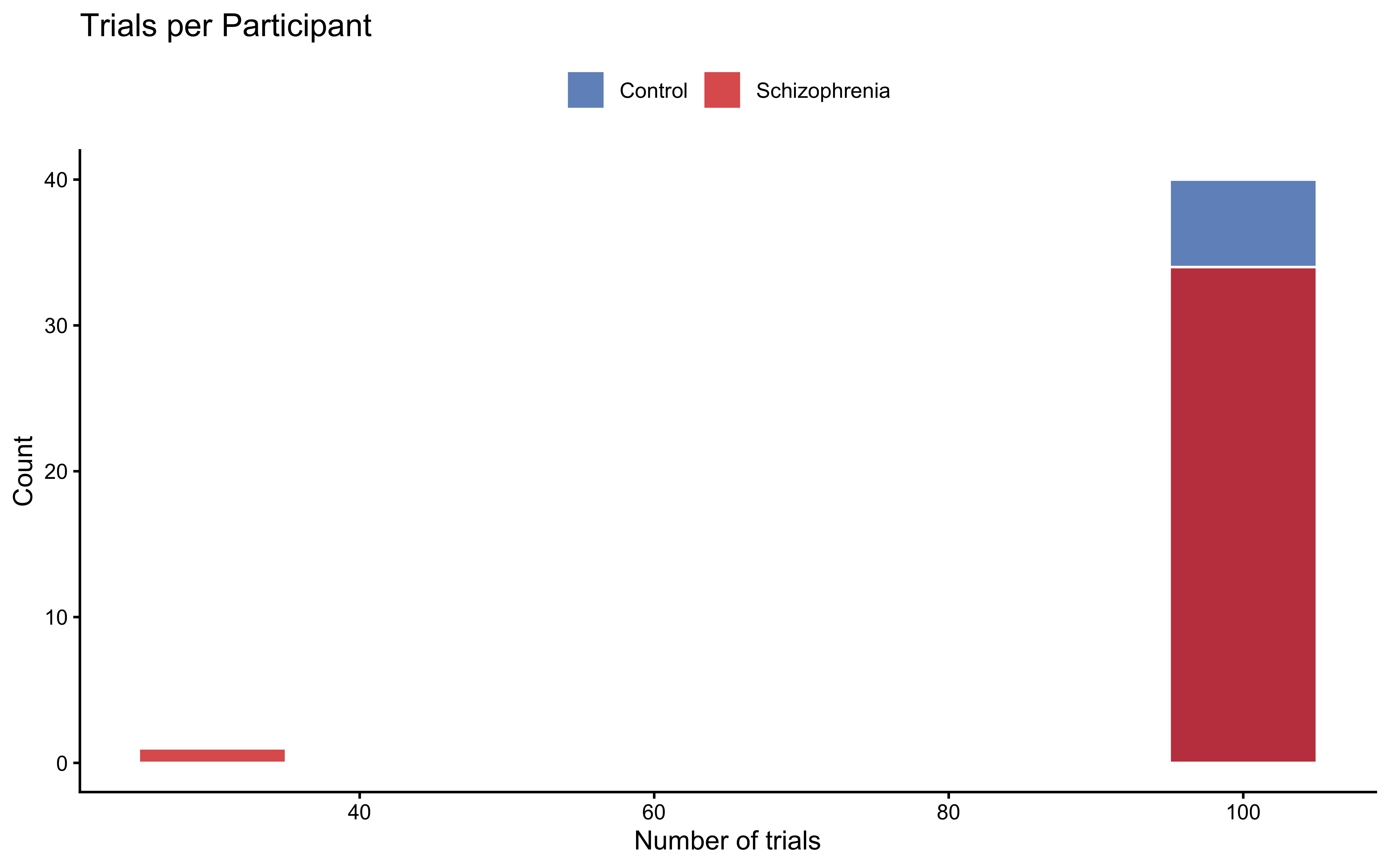
ggplot(trials_per_pp, aes(x = n_trials, fill = group_label)) +
geom_histogram(binwidth = 10, colour = "white", alpha = 0.8,
position = "identity") +
scale_fill_manual(values = pal_group) +
labs(
title = "Trials per Participant",
x = "Number of trials", y = "Count", fill = NULL
) +
theme(legend.position = "top")
```
#### Evidence Distributions
```{r ch11b_explore_evidence, fig.height=4}
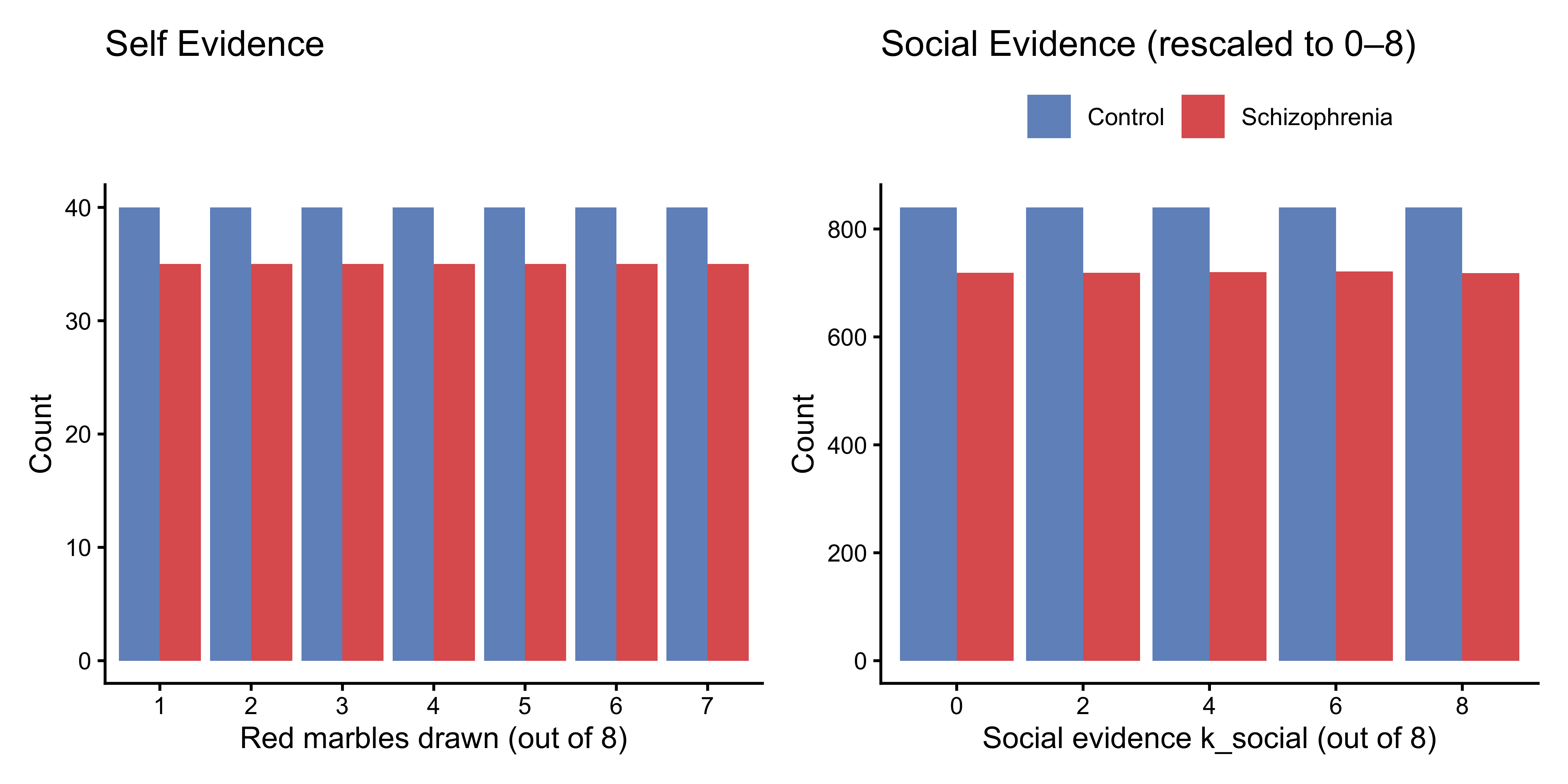
p_self_dist <- df |>
  distinct(participant, k_self, group_label) |>
  count(k_self, group_label) |>
  ggplot(aes(x = factor(k_self), y = n, fill = group_label)) +
  geom_col(position = "dodge", alpha = 0.8) +
  scale_fill_manual(values = pal_group) +
  labs(title = "Self Evidence", x = "Red marbles drawn (out of 8)",
       y = "Count", fill = NULL) +
  theme(legend.position = "none")

p_social_dist <- df |>
  count(k_social, group_label) |>
  ggplot(aes(x = factor(k_social), y = n, fill = group_label)) +
  geom_col(position = "dodge", alpha = 0.8) +
  scale_fill_manual(values = pal_group) +
  labs(title = "Social Evidence (rescaled to 0–8)",
       x = "Social evidence k_social (out of 8)", y = "Count", fill = NULL) +
  theme(legend.position = "top")

p_self_dist + p_social_dist
```
#### Psychometric Curves
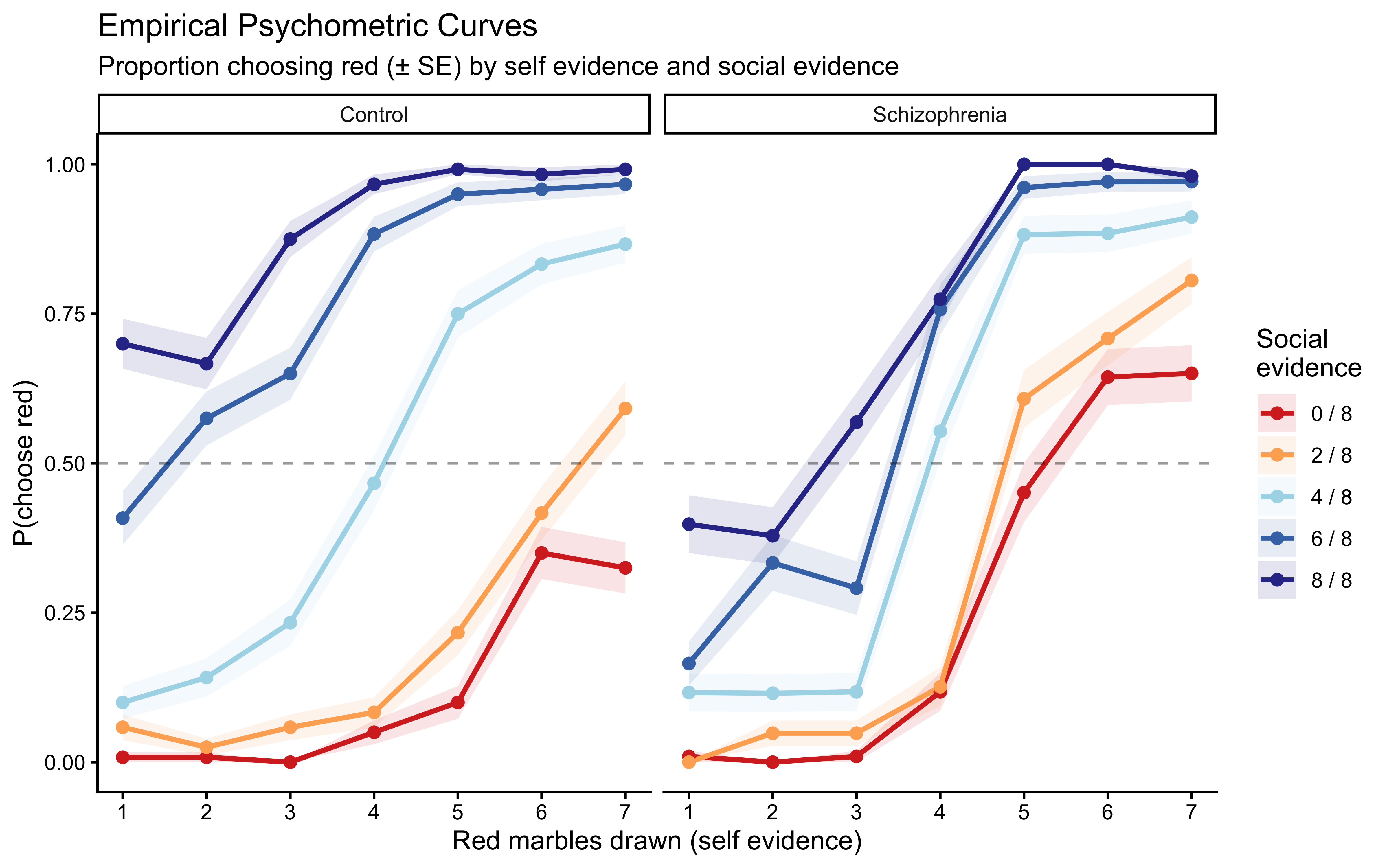
The most informative descriptive analysis is the **psychometric curve**: how does the probability of choosing red change with self evidence, for each level of social evidence?
```{r ch11b_psychometric, fig.height=5}
psycho_df <- df |>
  mutate(social_label = paste0(k_social, " / 8")) |>
  group_by(group_label, k_self, social_label) |>
  summarise(
    p_red  = mean(choice_red),
    n      = n(),
    se     = sqrt(p_red * (1 - p_red) / n),
    .groups = "drop"
  )

ggplot(psycho_df,
       aes(x = k_self, y = p_red,
           colour = social_label, group = social_label)) +
  geom_ribbon(aes(ymin = p_red - se, ymax = p_red + se,
                  fill = social_label),
              alpha = 0.12, colour = NA) +
  geom_line(linewidth = 1) +
  geom_point(size = 2) +
  geom_hline(yintercept = 0.5, linetype = "dashed", alpha = 0.4) +
  facet_wrap(~group_label) +
  scale_colour_manual(values = pal_social) +
  scale_fill_manual(values = pal_social) +
  scale_x_continuous(breaks = 1:7) +
  labs(
    title    = "Empirical Psychometric Curves",
    subtitle = "Proportion choosing red (± SE) by self evidence and social evidence",
    x        = "Red marbles drawn (self evidence)",
    y        = "P(choose red)",
    colour   = "Social\nevidence",
    fill     = "Social\nevidence"
  ) +
  theme(legend.position = "right")
```
Both groups show the expected main effects: more red self evidence increases P(choose red), and more social evidence for red shifts the curves upward. Patients appear to show steeper self-evidence curves (suggesting stronger self-weighting or overcounting) and somewhat compressed social-evidence separation (suggesting less social influence). We will quantify these impressions with models.
#### Overall Accuracy
```{r ch11b_accuracy}
df |>
  group_by(group_label, participant) |>
  summarise(acc = mean(choice_red == as.integer(
    (k_self / n_self + k_social / n_social) / 2 > 0.5)),
    .groups = "drop") |>
  group_by(group_label) |>
  summarise(mean_acc = mean(acc), sd_acc = sd(acc), .groups = "drop")
```
## Adapting Pseudo-Count Models to the Experimental Design
Chapter 11 derived and validated three pseudo-count Bayesian agents using the marble task's original encoding (direct evidence: 0–8 blue marbles out of 8; social evidence: 0–3 pseudo-marbles out of 3). The present dataset differs in two respects:
1. **Social evidence is aggregated from 4 binary responses.** We rescale to an equivalent 8-vote sample ($k_\text{social} \in \{0, 2, 4, 6, 8\}$, $n_\text{social} = 8$) so both sources can contribute the same maximum pseudo-counts in the SBA, making the SBA a genuine equal-weighting baseline and the WBA's $w_\text{self}/w_\text{social}$ ratio directly interpretable as relative trust.
2. **Extreme self-evidence values are absent** by design ($k_\text{self} \in \{1, \ldots, 7\}$, not $\{0, \ldots, 8\}$).
The model mathematics are unchanged; we pass the rescaled counts.
### Evidence Combinations for this Design
```{r ch11b_evidence_combinations}
# Social evidence levels after rescaling: 0×2, 1×2, 2×2, 3×2, 4×2
evidence_combinations <- expand_grid(
  k_self   = 1:7,
  k_social = c(0L, 2L, 4L, 6L, 8L),
  n_self   = 8L,
  n_social = 8L
)
cat("Unique evidence combinations:", nrow(evidence_combinations), "\n")
```
### Stan Models
#### Simple Bayesian Agent (SBA)
The SBA counts both sources at face value ($w_d = w_s = 1$, no free parameters). After rescaling, both use $n = 8$:
$$\alpha_\text{post} = 0.5 + k_\text{self} + k_\text{social}, \quad \beta_\text{post} = 0.5 + (8 - k_\text{self}) + (8 - k_\text{social})$$
```{r ch11b_stan_sba}
SBA_stan <- "
data {
  int<lower=1>                   N;
  array[N] int<lower=0, upper=1> y;
  array[N] int<lower=0>          k_self;
  array[N] int<lower=0>          n_self;
  array[N] int<lower=0>          k_social;
  array[N] int<lower=0>          n_social;
  int<lower=0, upper=1>          run_diagnostics;
}
model {
  vector[N] a = 0.5 + to_vector(k_self) + to_vector(k_social);
  vector[N] b = 0.5 + (to_vector(n_self)   - to_vector(k_self))
                    + (to_vector(n_social) - to_vector(k_social));
  target += beta_binomial_lpmf(y | 1, a, b);
}
generated quantities {
  vector[N] log_lik;
  array[N] int y_rep;
  if (run_diagnostics) {
    for (i in 1:N) {
      real a_i = 0.5 + k_self[i] + k_social[i];
      real b_i = 0.5 + (n_self[i] - k_self[i]) + (n_social[i] - k_social[i]);
      log_lik[i] = beta_binomial_lpmf(y[i] | 1, a_i, b_i);
      y_rep[i]   = beta_binomial_rng(1, a_i, b_i);
    }
  }
}
"
write_stan_file(SBA_stan, dir = "stan/", basename = "ch11b_sba.stan")
```
#### Proportional Bayesian Agent (PBA)
$p \in (0,1)$ allocates the unit evidence budget between self ($p$) and social ($1-p$):
```{r ch11b_stan_pba}
PBA_stan <- "
data {
  int<lower=1>                   N;
  array[N] int<lower=0, upper=1> y;
  array[N] int<lower=0>          k_self;
  array[N] int<lower=0>          n_self;
  array[N] int<lower=0>          k_social;
  array[N] int<lower=0>          n_social;
  real<lower=0>                  prior_p_alpha;
  real<lower=0>                  prior_p_beta;
  int<lower=0, upper=1>          run_diagnostics;
}
parameters {
  real<lower=0, upper=1> p;
}
model {
  target += beta_lpdf(p | prior_p_alpha, prior_p_beta);
  vector[N] a = 0.5 + p * to_vector(k_self)
                    + (1.0 - p) * to_vector(k_social);
  vector[N] b = 0.5 + p * (to_vector(n_self) - to_vector(k_self))
                    + (1.0 - p) * (to_vector(n_social) - to_vector(k_social));
  target += beta_binomial_lpmf(y | 1, a, b);
}
generated quantities {
  vector[N] log_lik;
  array[N] int y_rep;
  if (run_diagnostics) {
    for (i in 1:N) {
      real a_i = 0.5 + p * k_self[i] + (1.0 - p) * k_social[i];
      real b_i = 0.5 + p * (n_self[i] - k_self[i])
                     + (1.0 - p) * (n_social[i] - k_social[i]);
      log_lik[i] = beta_binomial_lpmf(y[i] | 1, a_i, b_i);
      y_rep[i]   = beta_binomial_rng(1, a_i, b_i);
    }
  }
}
"
write_stan_file(PBA_stan, dir = "stan/", basename = "ch11b_pba.stan")
```
#### Reparameterised Weighted Bayesian Agent (WBA)
$\rho$ (relative self-weight) and $\kappa$ (total evidence scale) resolve the ridge identifiability problem of the raw $w_d, w_s$ parameterisation (see Chapter 11):
```{r ch11b_stan_wba}
WBA_stan <- "
data {
  int<lower=1>                   N;
  array[N] int<lower=0, upper=1> y;
  array[N] int<lower=0>          k_self;
  array[N] int<lower=0>          n_self;
  array[N] int<lower=0>          k_social;
  array[N] int<lower=0>          n_social;
  real<lower=0>                  prior_rho_alpha;
  real<lower=0>                  prior_rho_beta;
  real                           prior_kappa_mu;
  real<lower=0>                  prior_kappa_sigma;
  int<lower=0, upper=1>          run_diagnostics;
}
parameters {
  real<lower=0, upper=1> rho;
  real<lower=0>          kappa;
}
transformed parameters {
  real w_self   = rho * kappa;
  real w_social = (1.0 - rho) * kappa;
}
model {
  target += beta_lpdf(rho | prior_rho_alpha, prior_rho_beta);
  target += lognormal_lpdf(kappa | prior_kappa_mu, prior_kappa_sigma);
  vector[N] a = 0.5 + w_self   * to_vector(k_self)
                    + w_social * to_vector(k_social);
  vector[N] b = 0.5 + w_self   * (to_vector(n_self)   - to_vector(k_self))
                    + w_social * (to_vector(n_social) - to_vector(k_social));
  target += beta_binomial_lpmf(y | 1, a, b);
}
generated quantities {
  vector[N] log_lik;
  array[N] int y_rep;
  if (run_diagnostics) {
    for (i in 1:N) {
      real a_i = 0.5 + w_self * k_self[i] + w_social * k_social[i];
      real b_i = 0.5 + w_self * (n_self[i] - k_self[i])
                     + w_social * (n_social[i] - k_social[i]);
      log_lik[i] = beta_binomial_lpmf(y[i] | 1, a_i, b_i);
      y_rep[i]   = beta_binomial_rng(1, a_i, b_i);
    }
  }
}
"
write_stan_file(WBA_stan, dir = "stan/", basename = "ch11b_wba.stan")
```
### Fitting the Pseudo-Count Models
```{r ch11b_compile_pseudocount}
mod_sba <- cmdstan_model("stan/ch11b_sba.stan", dir = "simmodels")
mod_pba <- cmdstan_model("stan/ch11b_pba.stan", dir = "simmodels")
mod_wba <- cmdstan_model("stan/ch11b_wba.stan", dir = "simmodels")
```
```{r ch11b_fit_pseudocount}
stan_data_base <- list(
  N          = nrow(df),
  y          = df$choice_red,
  k_self     = df$k_self,
  n_self     = df$n_self,
  k_social   = df$k_social,
  n_social   = df$n_social,
  run_diagnostics = 1L
)

if (regenerate_fits || !file.exists("simmodels/ch11b_sba_fit.rds")) {

  fit_sba <- mod_sba$sample(
    data = c(stan_data_base),
    chains = 4, parallel_chains = 4,
    iter_warmup = 1000, iter_sampling = 1000,
    refresh = 0
  )

  fit_pba <- mod_pba$sample(
    data = c(stan_data_base,
             list(prior_p_alpha = 2.0, prior_p_beta = 2.0)),
    chains = 4, parallel_chains = 4,
    iter_warmup = 1000, iter_sampling = 1000,
    refresh = 0
  )

  fit_wba <- mod_wba$sample(
    data = c(stan_data_base,
             list(prior_rho_alpha = 2.0, prior_rho_beta = 2.0,
                  prior_kappa_mu  = log(2), prior_kappa_sigma = 0.5)),
    chains = 4, parallel_chains = 4,
    iter_warmup = 1000, iter_sampling = 1000,
    refresh = 0
  )

  fit_sba$save_object("simmodels/ch11b_sba_fit.rds")
  fit_pba$save_object("simmodels/ch11b_pba_fit.rds")
  fit_wba$save_object("simmodels/ch11b_wba_fit.rds")

} else {
  fit_sba <- readRDS("simmodels/ch11b_sba_fit.rds")
  fit_pba <- readRDS("simmodels/ch11b_pba_fit.rds")
  fit_wba <- readRDS("simmodels/ch11b_wba_fit.rds")
}
```
### LOO Comparison of Pseudo-Count Models
```{r ch11b_loo_pseudocount}
loo_sba <- fit_sba$loo()
loo_pba <- fit_pba$loo()
loo_wba <- fit_wba$loo()

loo_compare(loo_sba, loo_pba, loo_wba)
```
```{r ch11b_pseudocount_params}
# PBA and WBA parameter posteriors
fit_pba$summary("p")
fit_wba$summary(c("rho", "kappa", "w_self", "w_social"))
```
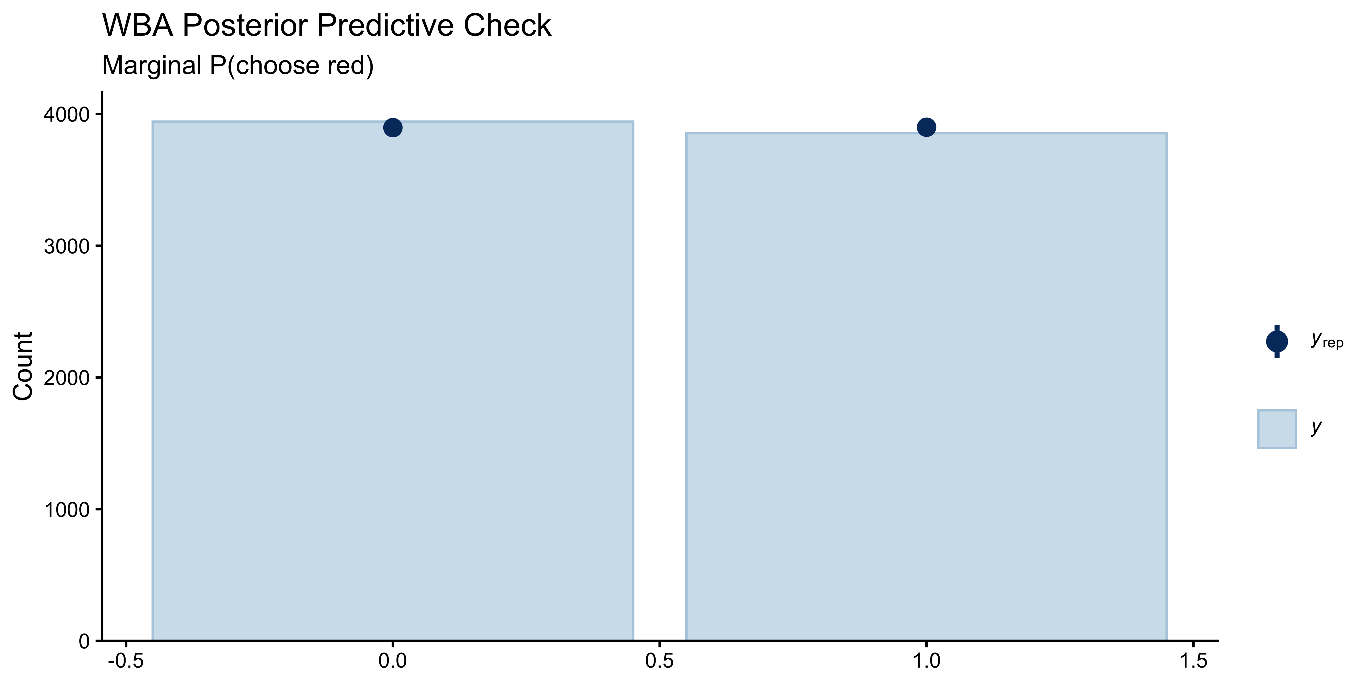
The WBA's reparameterised posterior shows $\rho > 0.5$, indicating that — pooled across all participants — self evidence receives more weight than social evidence. The LOO comparison will tell us whether this added flexibility actually improves out-of-sample predictive accuracy over the SBA.
### Prior and Posterior Predictive Check (Pseudo-Count)
```{r ch11b_ppc_pseudocount, fig.height=4}
y_rep_wba <- as_draws_matrix(fit_wba$draws("y_rep"))
n_rep      <- min(200, nrow(y_rep_wba))
y_rep_sub  <- y_rep_wba[sample(nrow(y_rep_wba), n_rep), ]

ppc_bars(y = df$choice_red, yrep = y_rep_sub) +
  labs(title = "WBA Posterior Predictive Check",
       subtitle = "Marginal P(choose red)")
```
## Log-Odds Models: Theory and Implementation
### The Jardri Transformation Function
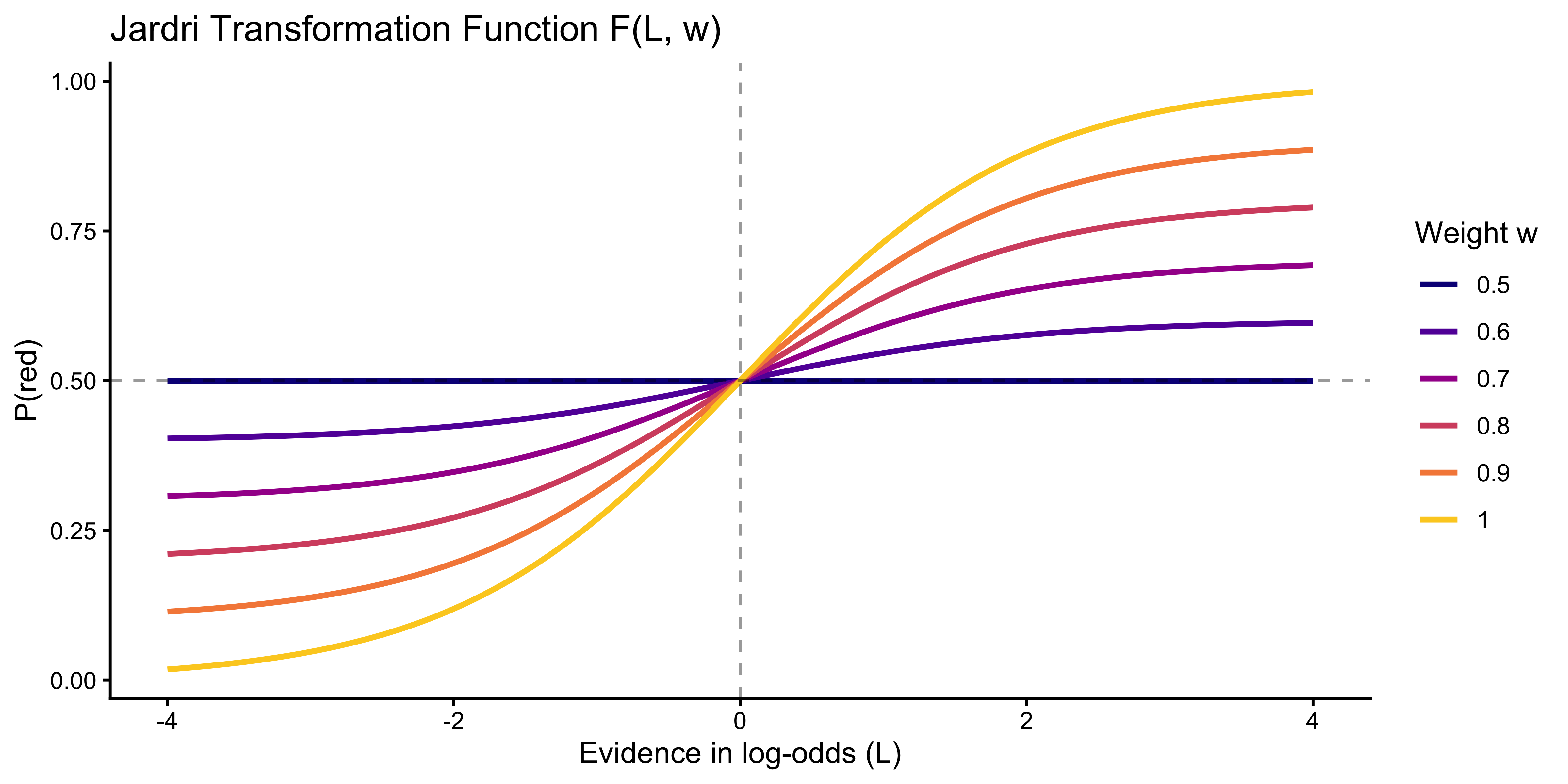
The pseudo-count agents operate on counts. To model *amplification* (overcounting), we must move to log-odds space. Define:
$$F(L, w) = \log \frac{w e^L + (1-w)}{(1-w) e^L + w}, \quad w \in [0.5, 1.0]$$
At $w = 1$, $F(L, 1) = L$ (full trust, evidence taken at face value). At $w = 0.5$, $F(L, 0.5) = 0$ (no trust, evidence ignored). The function is a smooth, bounded version of linear weighting.
```{r ch11b_jardri_viz, fig.height=4}
tibble(L = seq(-4, 4, by = 0.05)) |>
  expand_grid(w = c(0.5, 0.6, 0.7, 0.8, 0.9, 1.0)) |>
  mutate(FL = jardri_f(L, w), Prob = plogis(FL)) |>
  ggplot(aes(x = L, y = Prob, colour = factor(w))) +
  geom_line(linewidth = 1) +
  geom_hline(yintercept = 0.5, linetype = "dashed", alpha = 0.4) +
  geom_vline(xintercept = 0, linetype = "dashed", alpha = 0.4) +
  scale_colour_viridis_d(option = "plasma", end = 0.9) +
  labs(
    title  = "Jardri Transformation Function F(L, w)",
    x = "Evidence in log-odds (L)", y = "P(red)",
    colour = "Weight w"
  )
```
### The Four-Model Family
| Model | Parameters | Posterior log-odds |
|---|---|---|
| **Simple Bayes (SB)** | none | $L_1 + L_2$ |
| **Weighted Bayes (WB)** | $w_\text{s}, w_\text{o} \in [0.5, 1]$ | $F(L_1, w_\text{s}) + F(L_2, w_\text{o})$ |
| **CI (no interference)** | $w$'s + $\alpha_\text{s}, \alpha_\text{o} \geq 1$ | $F(\alpha_\text{s} L_1, w_\text{s}) + F(\alpha_\text{o} L_2, w_\text{o})$ |
| **CI (full)** | same + interference | $F(L_1 + I, w_\text{s}) + F(L_2 + I, w_\text{o})$, where $I = F(\alpha_\text{s} L_1, w_\text{s}) + F(\alpha_\text{o} L_2, w_\text{o})$ |
where $L_i = \log\!\left(\frac{0.5 + k_i}{0.5 + n_i - k_i}\right)$ (Jeffreys-smoothed log-odds) and the indices $\text{s}$ (self) and $\text{o}$ (other/social) replace the earlier $1$/$2$ notation.
All models use a Bernoulli data model: $y_i \sim \text{Bernoulli}(\sigma(L_\text{post}))$.
### Stan Implementation
#### Model 1: Simple Bayes (no free parameters)
```{r ch11b_stan_sb_lo}
SB_LO_stan <- "
data {
  int<lower=1>                   N;
  array[N] int<lower=0, upper=1> y;
  array[N] int<lower=0>          k_self;
  array[N] int<lower=0>          n_self;
  array[N] int<lower=0>          k_social;
  array[N] int<lower=0>          n_social;
  int<lower=0, upper=1>          run_diagnostics;
}
transformed data {
  real a0 = 0.5;
  real b0 = 0.5;
  array[N] real lo_self;
  array[N] real lo_social;
  for (i in 1:N) {
    lo_self[i]   = log((a0 + k_self[i])   / (b0 + n_self[i]   - k_self[i]));
    lo_social[i] = log((a0 + k_social[i]) / (b0 + n_social[i] - k_social[i]));
  }
}
model {
  for (i in 1:N)
    target += bernoulli_logit_lpmf(y[i] | lo_self[i] + lo_social[i]);
}
generated quantities {
  vector[N] log_lik;
  array[N] int y_rep;
  if (run_diagnostics) {
    for (i in 1:N) {
      real L = lo_self[i] + lo_social[i];
      log_lik[i] = bernoulli_logit_lpmf(y[i] | L);
      y_rep[i]   = bernoulli_logit_rng(L);
    }
  }
}
"
write_stan_file(SB_LO_stan, dir = "stan/", basename = "ch11b_sb_lo.stan")
```
#### Model 2: Weighted Bayes
```{r ch11b_stan_wb_lo}
WB_LO_stan <- "
functions {
  real jardri_f(real L, real w) {
    real num = w * exp(L) + (1.0 - w);
    real den = (1.0 - w) * exp(L) + w;
    return log(num / den);
  }
}
data {
  int<lower=1>                   N;
  array[N] int<lower=0, upper=1> y;
  array[N] int<lower=0>          k_self;
  array[N] int<lower=0>          n_self;
  array[N] int<lower=0>          k_social;
  array[N] int<lower=0>          n_social;
  int<lower=0, upper=1>          run_diagnostics;
}
transformed data {
  real a0 = 0.5;
  real b0 = 0.5;
  array[N] real lo_self;
  array[N] real lo_social;
  for (i in 1:N) {
    lo_self[i]   = log((a0 + k_self[i])   / (b0 + n_self[i]   - k_self[i]));
    lo_social[i] = log((a0 + k_social[i]) / (b0 + n_social[i] - k_social[i]));
  }
}
parameters {
  real<lower=0.5, upper=1.0> w_self;
  real<lower=0.5, upper=1.0> w_social;
}
model {
  w_self   ~ normal(0.75, 0.25);
  w_social ~ normal(0.75, 0.25);
  for (i in 1:N)
    target += bernoulli_logit_lpmf(y[i] |
                jardri_f(lo_self[i], w_self) + jardri_f(lo_social[i], w_social));
}
generated quantities {
  vector[N] log_lik;
  array[N] int y_rep;
  if (run_diagnostics) {
    for (i in 1:N) {
      real L = jardri_f(lo_self[i], w_self) + jardri_f(lo_social[i], w_social);
      log_lik[i] = bernoulli_logit_lpmf(y[i] | L);
      y_rep[i]   = bernoulli_logit_rng(L);
    }
  }
}
"
write_stan_file(WB_LO_stan, dir = "stan/", basename = "ch11b_wb_lo.stan")
```
#### Model 3: Circular Inference without Interference
```{r ch11b_stan_ci_loops}
CI_Loops_stan <- "
functions {
  real jardri_f(real L, real w) {
    real num = w * exp(L) + (1.0 - w);
    real den = (1.0 - w) * exp(L) + w;
    return log(num / den);
  }
}
data {
  int<lower=1>                   N;
  array[N] int<lower=0, upper=1> y;
  array[N] int<lower=0>          k_self;
  array[N] int<lower=0>          n_self;
  array[N] int<lower=0>          k_social;
  array[N] int<lower=0>          n_social;
  int<lower=0, upper=1>          run_diagnostics;
}
transformed data {
  real a0 = 0.5;
  real b0 = 0.5;
  array[N] real lo_self;
  array[N] real lo_social;
  for (i in 1:N) {
    lo_self[i]   = log((a0 + k_self[i])   / (b0 + n_self[i]   - k_self[i]));
    lo_social[i] = log((a0 + k_social[i]) / (b0 + n_social[i] - k_social[i]));
  }
}
parameters {
  real<lower=0.5, upper=1.0> w_self;
  real<lower=0.5, upper=1.0> w_social;
  real<lower=0>              alpha_self_m1;    // excess over 1
  real<lower=0>              alpha_social_m1;
}
transformed parameters {
  real<lower=1> alpha_self   = 1.0 + alpha_self_m1;
  real<lower=1> alpha_social = 1.0 + alpha_social_m1;
}
model {
  w_self   ~ normal(0.75, 0.25);
  w_social ~ normal(0.75, 0.25);
  alpha_self_m1   ~ std_normal();
  alpha_social_m1 ~ std_normal();
  for (i in 1:N)
    target += bernoulli_logit_lpmf(y[i] |
                jardri_f(alpha_self   * lo_self[i],   w_self) +
                jardri_f(alpha_social * lo_social[i], w_social));
}
generated quantities {
  vector[N] log_lik;
  array[N] int y_rep;
  if (run_diagnostics) {
    for (i in 1:N) {
      real L = jardri_f(alpha_self   * lo_self[i],   w_self) +
               jardri_f(alpha_social * lo_social[i], w_social);
      log_lik[i] = bernoulli_logit_lpmf(y[i] | L);
      y_rep[i]   = bernoulli_logit_rng(L);
    }
  }
}
"
write_stan_file(CI_Loops_stan, dir = "stan/", basename = "ch11b_ci_loops.stan")
```
#### Model 4: Circular Inference with Interference (Full Jardri Model)
```{r ch11b_stan_ci_full}
CI_Full_stan <- "
functions {
  real jardri_f(real L, real w) {
    real num = w * exp(L) + (1.0 - w);
    real den = (1.0 - w) * exp(L) + w;
    return log(num / den);
  }
}
data {
  int<lower=1>                   N;
  array[N] int<lower=0, upper=1> y;
  array[N] int<lower=0>          k_self;
  array[N] int<lower=0>          n_self;
  array[N] int<lower=0>          k_social;
  array[N] int<lower=0>          n_social;
  int<lower=0, upper=1>          run_diagnostics;
}
transformed data {
  real a0 = 0.5;
  real b0 = 0.5;
  array[N] real lo_self;
  array[N] real lo_social;
  for (i in 1:N) {
    lo_self[i]   = log((a0 + k_self[i])   / (b0 + n_self[i]   - k_self[i]));
    lo_social[i] = log((a0 + k_social[i]) / (b0 + n_social[i] - k_social[i]));
  }
}
parameters {
  real<lower=0.5, upper=1.0> w_self;
  real<lower=0.5, upper=1.0> w_social;
  real<lower=0>              alpha_self_m1;
  real<lower=0>              alpha_social_m1;
}
transformed parameters {
  real<lower=1> alpha_self   = 1.0 + alpha_self_m1;
  real<lower=1> alpha_social = 1.0 + alpha_social_m1;
}
model {
  w_self   ~ normal(0.75, 0.25);
  w_social ~ normal(0.75, 0.25);
  alpha_self_m1   ~ std_normal();
  alpha_social_m1 ~ std_normal();
  for (i in 1:N) {
    real I = jardri_f(alpha_self   * lo_self[i],   w_self) +
             jardri_f(alpha_social * lo_social[i], w_social);
    real L = jardri_f(lo_self[i]   + I, w_self) +
             jardri_f(lo_social[i] + I, w_social);
    target += bernoulli_logit_lpmf(y[i] | L);
  }
}
generated quantities {
  vector[N] log_lik;
  array[N] int y_rep;
  if (run_diagnostics) {
    for (i in 1:N) {
      real I = jardri_f(alpha_self   * lo_self[i],   w_self) +
               jardri_f(alpha_social * lo_social[i], w_social);
      real L = jardri_f(lo_self[i]   + I, w_self) +
               jardri_f(lo_social[i] + I, w_social);
      log_lik[i] = bernoulli_logit_lpmf(y[i] | L);
      y_rep[i]   = bernoulli_logit_rng(L);
    }
  }
}
"
write_stan_file(CI_Full_stan, dir = "stan/", basename = "ch11b_ci_full.stan")
```
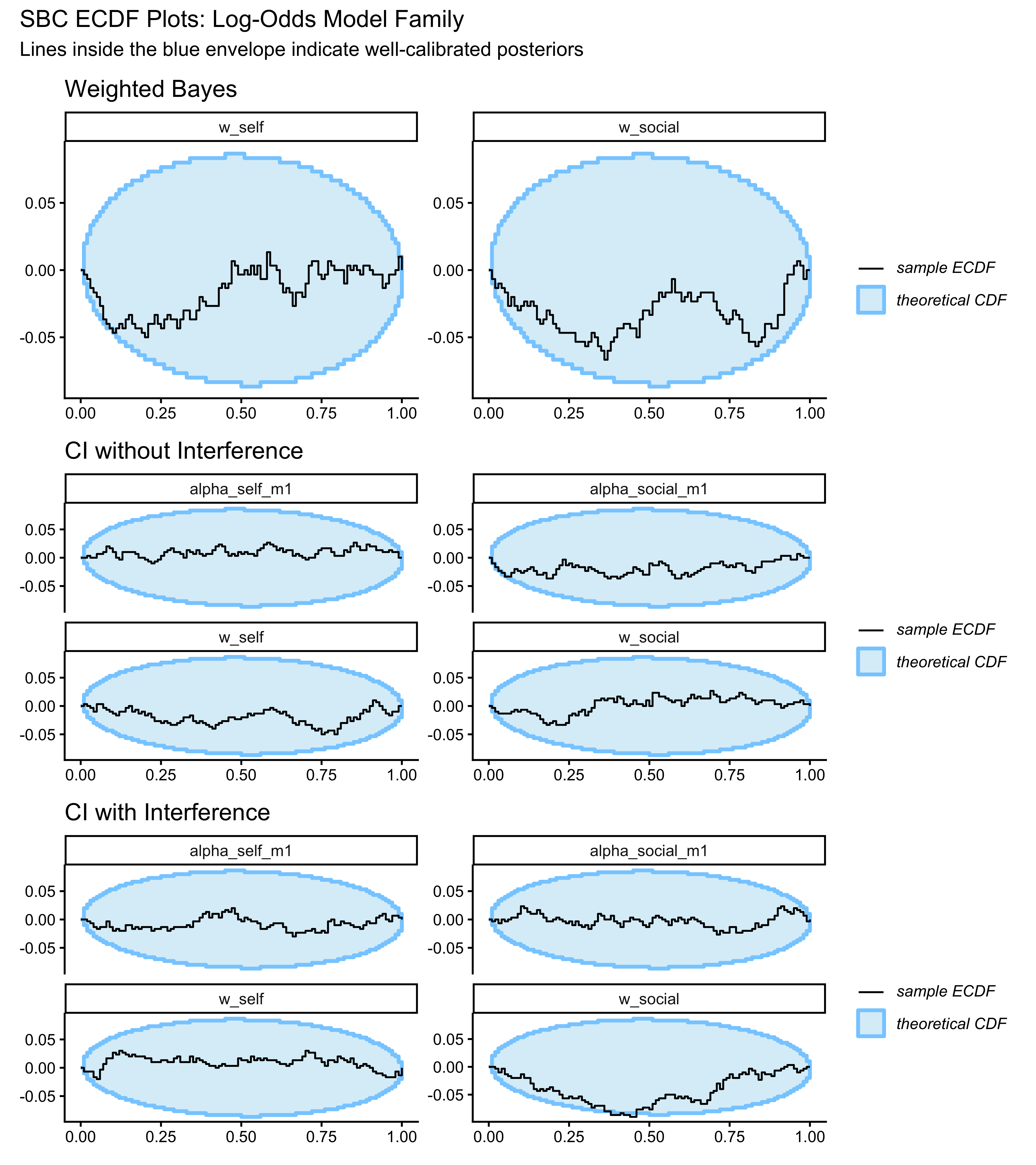
## Validation: Simulation-Based Calibration Checks
Before fitting to empirical data we need confidence that our Stan samplers can recover parameters without bias. We run Simulation-Based Calibration Checks (SBC) on the three models with free parameters (WB, CI-Loops, CI-Full). The parameter-free SB model requires no SBC.
For each model we:
1. Draw parameters from the prior.
2. Simulate a dataset of 210 trials (6 repetitions of 35 evidence combinations) using those parameters and the actual experimental design.
3. Fit the model to that simulated dataset.
4. Check whether the true parameter lies within the expected rank-quantile band.
```{r ch11b_compile_lo_models}
mod_sb_lo  <- cmdstan_model("stan/ch11b_sb_lo.stan",    dir = "simmodels")
mod_wb_lo  <- cmdstan_model("stan/ch11b_wb_lo.stan",    dir = "simmodels")
mod_ci_lo  <- cmdstan_model("stan/ch11b_ci_loops.stan", dir = "simmodels")
mod_cif_lo <- cmdstan_model("stan/ch11b_ci_full.stan",  dir = "simmodels")
```
```{r ch11b_sbc_generators}
N_sbc_trials <- nrow(evidence_combinations) * 6L  # 210 trials

draw_w <- function() {
  w <- -1
  while (w < 0.5 || w > 1.0) w <- rnorm(1, 0.75, 0.25)
  w
}

make_sbc_data <- function(ev, lo_s, lo_o, L_post) {
  list(
    N        = nrow(ev),
    y        = rbinom(nrow(ev), 1, plogis(L_post)),
    k_self   = ev$k_self,   n_self   = ev$n_self,
    k_social = ev$k_social, n_social = ev$n_social,
    run_diagnostics = 0L
  )
}

sbc_gen_wb <- SBC_generator_function(
  function(N) {
    ws <- draw_w(); wo <- draw_w()
    ev <- evidence_combinations |> slice_sample(n = N, replace = TRUE)
    lo_s <- log((0.5 + ev$k_self)   / (0.5 + ev$n_self   - ev$k_self))
    lo_o <- log((0.5 + ev$k_social) / (0.5 + ev$n_social - ev$k_social))
    L    <- jardri_f(lo_s, ws) + jardri_f(lo_o, wo)
    list(
      variables = list(w_self = ws, w_social = wo),
      generated = make_sbc_data(ev, lo_s, lo_o, L)
    )
  }, N = N_sbc_trials
)

sbc_gen_ci <- SBC_generator_function(
  function(N) {
    ws <- draw_w(); wo <- draw_w()
    as_m1 <- abs(rnorm(1, 0, 1)); ao_m1 <- abs(rnorm(1, 0, 1))
    as <- 1 + as_m1; ao <- 1 + ao_m1
    ev <- evidence_combinations |> slice_sample(n = N, replace = TRUE)
    lo_s <- log((0.5 + ev$k_self)   / (0.5 + ev$n_self   - ev$k_self))
    lo_o <- log((0.5 + ev$k_social) / (0.5 + ev$n_social - ev$k_social))
    L    <- jardri_f(as * lo_s, ws) + jardri_f(ao * lo_o, wo)
    list(
      variables = list(w_self = ws, w_social = wo,
                       alpha_self_m1 = as_m1, alpha_social_m1 = ao_m1),
      generated = make_sbc_data(ev, lo_s, lo_o, L)
    )
  }, N = N_sbc_trials
)

sbc_gen_cif <- SBC_generator_function(
  function(N) {
    ws <- draw_w(); wo <- draw_w()
    as_m1 <- abs(rnorm(1, 0, 1)); ao_m1 <- abs(rnorm(1, 0, 1))
    as <- 1 + as_m1; ao <- 1 + ao_m1
    ev <- evidence_combinations |> slice_sample(n = N, replace = TRUE)
    lo_s <- log((0.5 + ev$k_self)   / (0.5 + ev$n_self   - ev$k_self))
    lo_o <- log((0.5 + ev$k_social) / (0.5 + ev$n_social - ev$k_social))
    I    <- jardri_f(as * lo_s, ws) + jardri_f(ao * lo_o, wo)
    L    <- jardri_f(lo_s + I, ws) + jardri_f(lo_o + I, wo)
    list(
      variables = list(w_self = ws, w_social = wo,
                       alpha_self_m1 = as_m1, alpha_social_m1 = ao_m1),
      generated = make_sbc_data(ev, lo_s, lo_o, L)
    )
  }, N = N_sbc_trials
)
```
```{r ch11b_run_sbc}
if (regenerate_sbc || !file.exists("simmodels/ch11b_sbc_results.rds")) {

  n_sbc <- 300
  sampler_args <- list(
    chains = 2, iter_warmup = 500, iter_sampling = 500,
    parallel_chains = 2, refresh = 0
  )

  ds_wb  <- generate_datasets(sbc_gen_wb,  n_sbc)
  ds_ci  <- generate_datasets(sbc_gen_ci,  n_sbc)
  ds_cif <- generate_datasets(sbc_gen_cif, n_sbc)

  be_wb  <- do.call(SBC_backend_cmdstan_sample, c(list(model = mod_wb_lo),  sampler_args))
  be_ci  <- do.call(SBC_backend_cmdstan_sample, c(list(model = mod_ci_lo),  sampler_args))
  be_cif <- do.call(SBC_backend_cmdstan_sample, c(list(model = mod_cif_lo), sampler_args))

  sbc_wb  <- compute_SBC(ds_wb,  be_wb,  keep_fits = FALSE)
  sbc_ci  <- compute_SBC(ds_ci,  be_ci,  keep_fits = FALSE)
  sbc_cif <- compute_SBC(ds_cif, be_cif, keep_fits = FALSE)

  saveRDS(list(wb = sbc_wb, ci = sbc_ci, cif = sbc_cif),
          "simmodels/ch11b_sbc_results.rds")

} else {
  sbc_all <- readRDS("simmodels/ch11b_sbc_results.rds")
  sbc_wb  <- sbc_all$wb
  sbc_ci  <- sbc_all$ci
  sbc_cif <- sbc_all$cif
}
```
### ECDF Calibration Plots
```{r ch11b_sbc_ecdf, fig.height=9}
p_ecdf_wb <- plot_ecdf_diff(sbc_wb, variables = c("w_self", "w_social")) +
  labs(title = "Weighted Bayes")

p_ecdf_ci <- plot_ecdf_diff(sbc_ci,
               variables = c("w_self", "w_social",
                             "alpha_self_m1", "alpha_social_m1")) +
  labs(title = "CI without Interference")

p_ecdf_cif <- plot_ecdf_diff(sbc_cif,
                variables = c("w_self", "w_social",
                              "alpha_self_m1", "alpha_social_m1")) +
  labs(title = "CI with Interference")

(p_ecdf_wb / p_ecdf_ci / p_ecdf_cif) +
  plot_annotation(
    title    = "SBC ECDF Plots: Log-Odds Model Family",
    subtitle = "Lines inside the blue envelope indicate well-calibrated posteriors"
  )
```
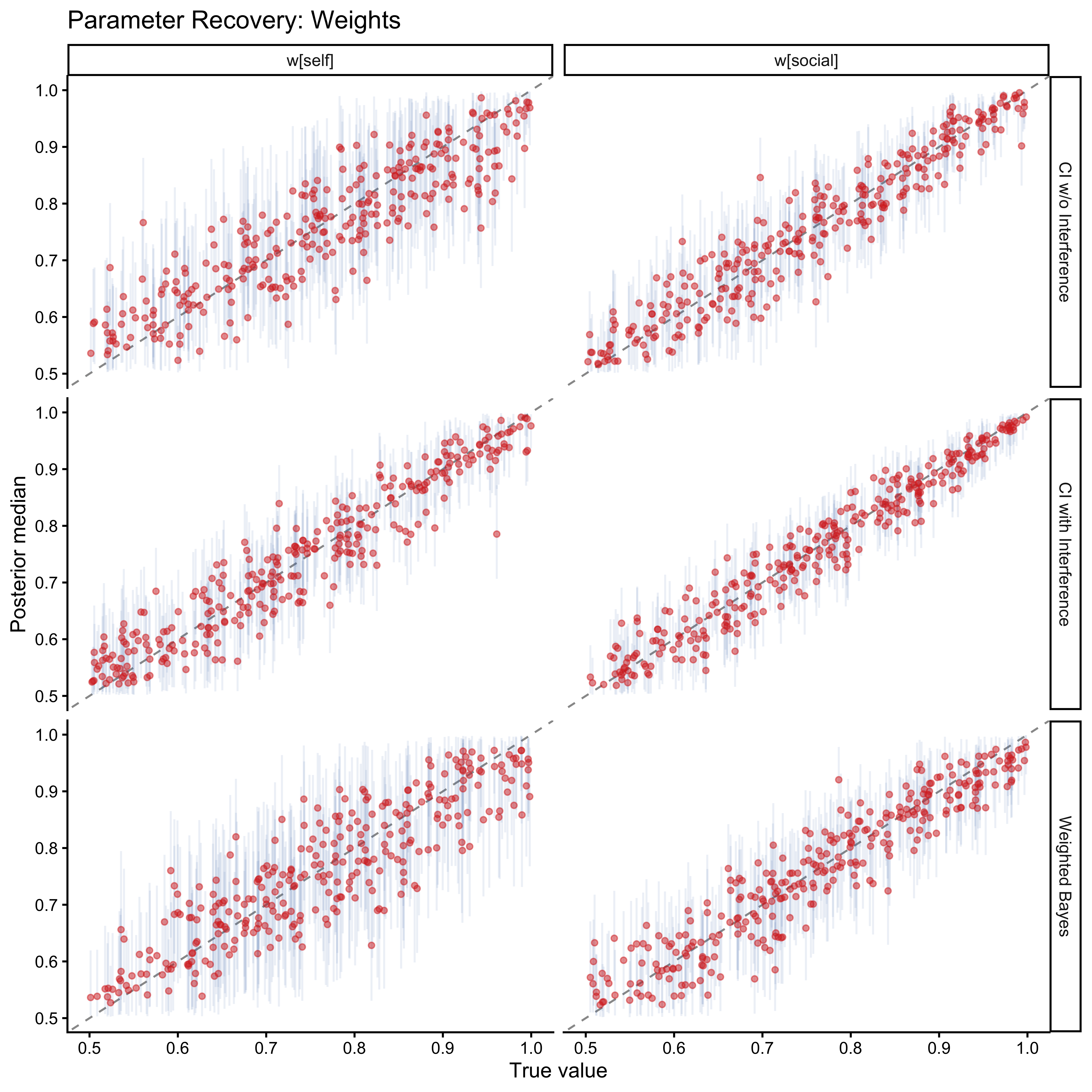
### Parameter Recovery
```{r ch11b_sbc_recovery, fig.height=8}
prep_rec <- function(sbc_obj, model_name) {
  sbc_obj$stats |>
    filter(variable %in% c("w_self", "w_social",
                            "alpha_self_m1", "alpha_social_m1")) |>
    mutate(
      model = model_name,
      param = recode(variable,
        w_self           = "w[self]",
        w_social         = "w[social]",
        alpha_self_m1    = "α[self] - 1",
        alpha_social_m1  = "α[social] - 1"
      )
    )
}

rec_df <- bind_rows(
  prep_rec(sbc_wb,  "Weighted Bayes"),
  prep_rec(sbc_ci,  "CI w/o Interference"),
  prep_rec(sbc_cif, "CI with Interference")
)

# Weights
rec_df |>
  filter(str_starts(variable, "w_")) |>
  ggplot(aes(x = simulated_value, y = median)) +
  geom_abline(linetype = "dashed", colour = "grey60") +
  geom_errorbar(aes(ymin = q5, ymax = q95), alpha = 0.1,
                width = 0, colour = "#4575b4") +
  geom_point(alpha = 0.5, size = 1.2, colour = "#d73027") +
  facet_grid(model ~ param) +
  coord_cartesian(xlim = c(0.5, 1), ylim = c(0.5, 1)) +
  labs(
    title = "Parameter Recovery: Weights",
    x = "True value", y = "Posterior median"
  )
```
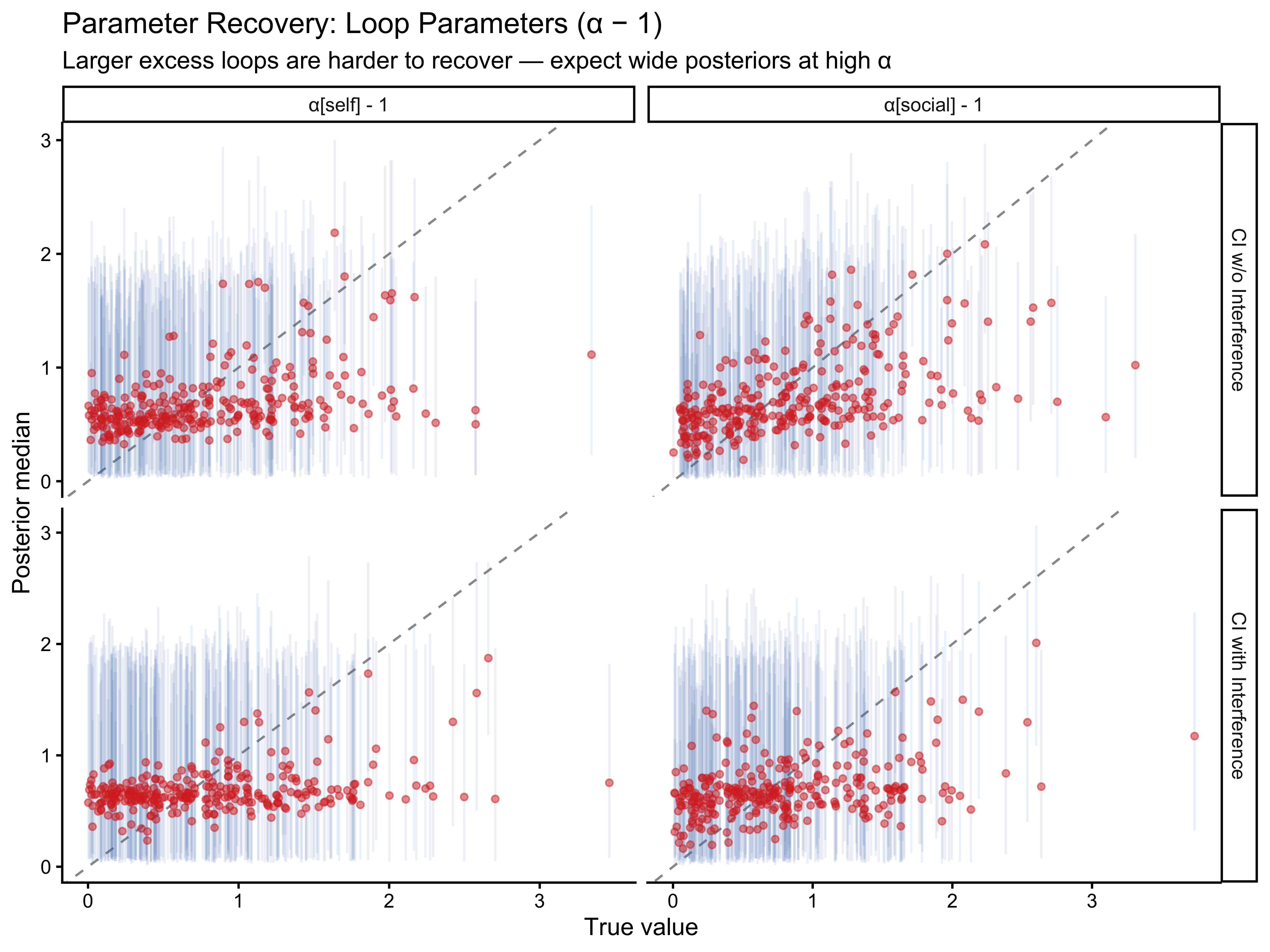
```{r ch11b_sbc_recovery_alpha, fig.height=6}
rec_df |>
  filter(str_starts(variable, "alpha_")) |>
  ggplot(aes(x = simulated_value, y = median)) +
  geom_abline(linetype = "dashed", colour = "grey60") +
  geom_errorbar(aes(ymin = q5, ymax = q95), alpha = 0.1,
                width = 0, colour = "#4575b4") +
  geom_point(alpha = 0.5, size = 1.2, colour = "#d73027") +
  facet_grid(model ~ param, scales = "free") +
  labs(
    title    = "Parameter Recovery: Loop Parameters (α − 1)",
    subtitle = "Larger excess loops are harder to recover — expect wide posteriors at high α",
    x = "True value", y = "Posterior median"
  )
```
Weights recover well across all models. Loop parameters become increasingly uncertain for large values: when $\alpha$ is large, the Jardri function saturates, and further increases in $\alpha$ produce no additional behavioural signal. This asymptote limits precision at the upper tail but does not introduce bias for the moderate values expected in human participants.
## Fitting to Empirical Data
### Compile and Fit All Four Models
```{r ch11b_fit_lo_models}
stan_data_lo <- list(
  N        = nrow(df),
  y        = df$choice_red,
  k_self   = df$k_self,   n_self   = df$n_self,
  k_social = df$k_social, n_social = df$n_social,
  run_diagnostics = 1L
)

if (regenerate_fits || !file.exists("simmodels/ch11b_sb_lo_fit.rds")) {

  sampler <- list(chains = 4, parallel_chains = 4,
                  iter_warmup = 1000, iter_sampling = 1000, refresh = 0)

  fit_sb_lo  <- do.call(mod_sb_lo$sample,  c(list(data = stan_data_lo), sampler))
  fit_wb_lo  <- do.call(mod_wb_lo$sample,  c(list(data = stan_data_lo), sampler))
  fit_ci_lo  <- do.call(mod_ci_lo$sample,  c(list(data = stan_data_lo), sampler))
  fit_cif_lo <- do.call(mod_cif_lo$sample, c(list(data = stan_data_lo), sampler))

  fit_sb_lo$save_object("simmodels/ch11b_sb_lo_fit.rds")
  fit_wb_lo$save_object("simmodels/ch11b_wb_lo_fit.rds")
  fit_ci_lo$save_object("simmodels/ch11b_ci_lo_fit.rds")
  fit_cif_lo$save_object("simmodels/ch11b_cif_lo_fit.rds")

} else {
  fit_sb_lo  <- readRDS("simmodels/ch11b_sb_lo_fit.rds")
  fit_wb_lo  <- readRDS("simmodels/ch11b_wb_lo_fit.rds")
  fit_ci_lo  <- readRDS("simmodels/ch11b_ci_lo_fit.rds")
  fit_cif_lo <- readRDS("simmodels/ch11b_cif_lo_fit.rds")
}
```
### Diagnostics
```{r ch11b_diagnostics}
for (nm in c("SB", "WB", "CI-Loops", "CI-Full")) {
  fit <- list(SB = fit_sb_lo, WB = fit_wb_lo,
              `CI-Loops` = fit_ci_lo, `CI-Full` = fit_cif_lo)[[nm]]
  dg  <- fit$diagnostic_summary(quiet = TRUE)
  cat(nm, "— divergences:", sum(dg$num_divergent),
      " max Rhat:", round(max(fit$summary()$rhat, na.rm = TRUE), 3), "\n")
}
```
### LOO Model Comparison
```{r ch11b_loo_lo_models}
loo_sb_lo  <- fit_sb_lo$loo()
loo_wb_lo  <- fit_wb_lo$loo()
loo_ci_lo  <- fit_ci_lo$loo()
loo_cif_lo <- fit_cif_lo$loo()

loo_tab <- loo_compare(loo_sb_lo, loo_wb_lo, loo_ci_lo, loo_cif_lo)
print(loo_tab, simplify = FALSE)
```
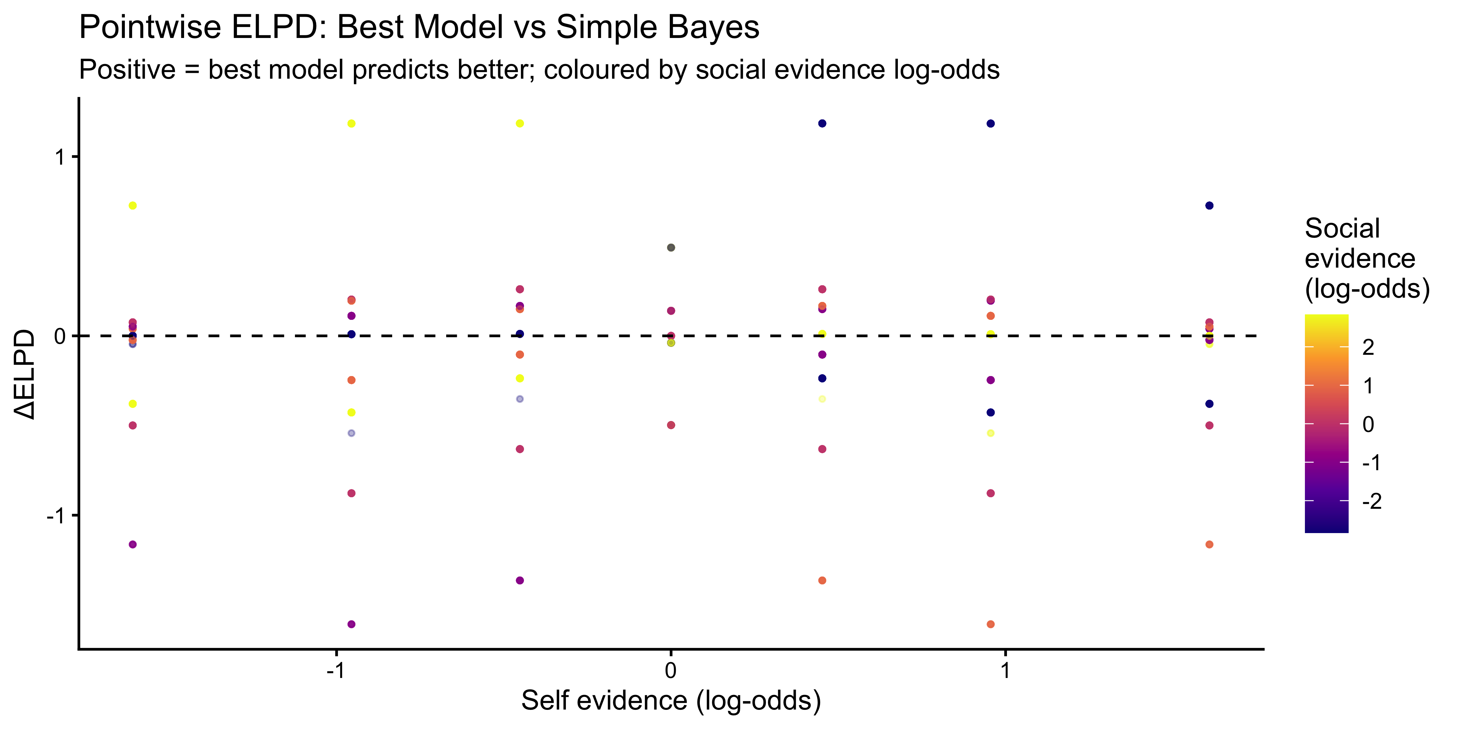
```{r ch11b_loo_plot, fig.height=4}
# Pointwise ELPD advantage of best model over SB
best_idx <- which.max(c(loo_sb_lo$estimates["elpd_loo","Estimate"],
                         loo_wb_lo$estimates["elpd_loo","Estimate"],
                         loo_ci_lo$estimates["elpd_loo","Estimate"],
                         loo_cif_lo$estimates["elpd_loo","Estimate"]))

best_fit <- list(fit_sb_lo, fit_wb_lo, fit_ci_lo, fit_cif_lo)[[best_idx]]
best_loo <- list(loo_sb_lo, loo_wb_lo, loo_ci_lo, loo_cif_lo)[[best_idx]]

# Compare pointwise ELPD: best vs SB
pw_diff <- best_loo$pointwise[, "elpd_loo"] -
           loo_sb_lo$pointwise[, "elpd_loo"]

tibble(
  diff = pw_diff,
  lo_self   = df$lo_self,
  lo_social = df$lo_social
) |>
  ggplot(aes(x = lo_self, y = diff, colour = lo_social)) +
  geom_point(alpha = 0.3, size = 0.8) +
  geom_hline(yintercept = 0, linetype = "dashed") +
  geom_smooth(colour = "black", linewidth = 0.8, se = FALSE) +
  scale_colour_viridis_c(option = "plasma") +
  labs(
    title    = "Pointwise ELPD: Best Model vs Simple Bayes",
    subtitle = "Positive = best model predicts better; coloured by social evidence log-odds",
    x        = "Self evidence (log-odds)", y = "ΔELPD",
    colour   = "Social\nevidence\n(log-odds)"
  )
```
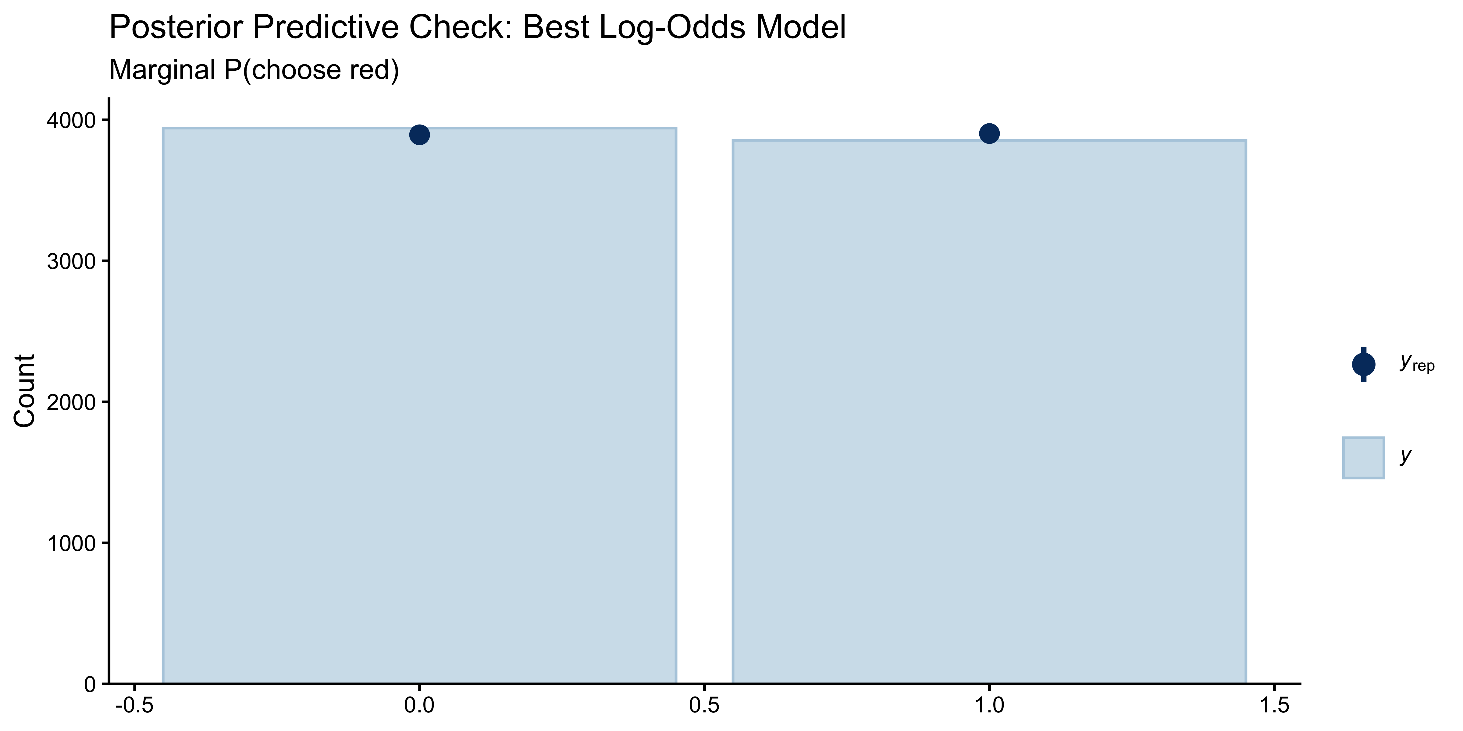
### Posterior Predictive Checks
```{r ch11b_ppc_lo, fig.height=4}
y_rep_best <- as_draws_matrix(best_fit$draws("y_rep"))
n_sub      <- min(200, nrow(y_rep_best))

ppc_bars(df$choice_red, y_rep_best[sample(nrow(y_rep_best), n_sub), ]) +
  labs(title = "Posterior Predictive Check: Best Log-Odds Model",
       subtitle = "Marginal P(choose red)")
```
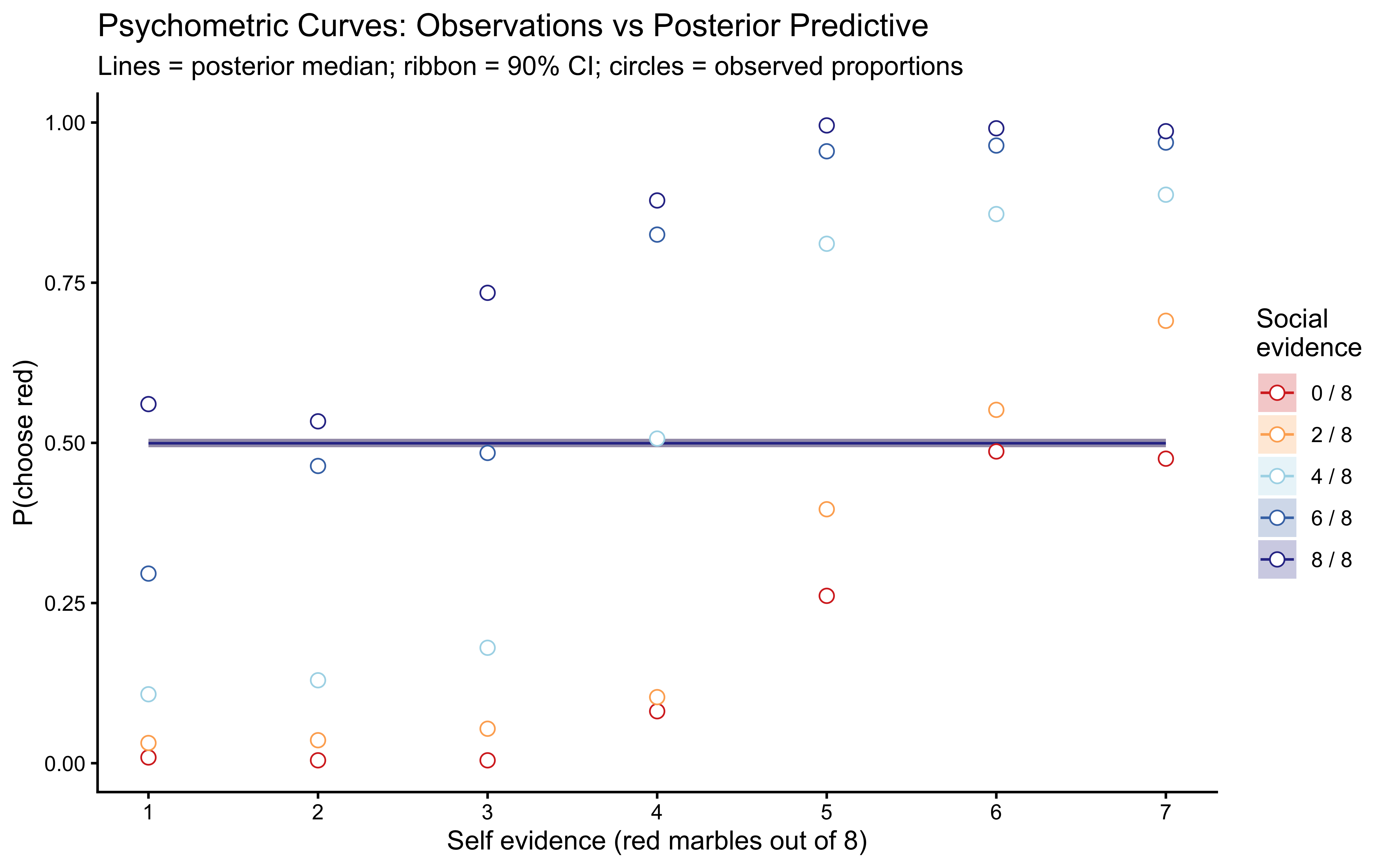
```{r ch11b_ppc_psychometric, fig.height=5}
# Predicted psychometric curves from posterior predictive
y_rep_mat   <- y_rep_best[sample(nrow(y_rep_best), 100), ]
pred_curves <- map_dfr(seq_len(nrow(y_rep_mat)), function(r) {
  df |>
    mutate(y_rep = y_rep_mat[r, ]) |>
    mutate(social_label = paste0(k_social, " / 8")) |>
    group_by(k_self, social_label) |>
    summarise(p_red = mean(y_rep), .groups = "drop") |>
    mutate(rep = r)
})

pred_summary <- pred_curves |>
  group_by(k_self, social_label) |>
  summarise(
    lo = quantile(p_red, 0.05),
    hi = quantile(p_red, 0.95),
    med = median(p_red),
    .groups = "drop"
  )

obs_curves <- df |>
  mutate(social_label = paste0(k_social, " / 8")) |>
  group_by(k_self, social_label) |>
  summarise(p_red = mean(choice_red), .groups = "drop")

ggplot() +
  geom_ribbon(data = pred_summary,
              aes(x = k_self, ymin = lo, ymax = hi,
                  fill = social_label), alpha = 0.25) +
  geom_line(data = pred_summary,
            aes(x = k_self, y = med, colour = social_label)) +
  geom_point(data = obs_curves,
             aes(x = k_self, y = p_red, colour = social_label),
             size = 2.5, shape = 21,
             fill = "white") +
  scale_colour_manual(values = pal_social) +
  scale_fill_manual(values = pal_social) +
  scale_x_continuous(breaks = 1:7) +
  labs(
    title    = "Psychometric Curves: Observations vs Posterior Predictive",
    subtitle = "Lines = posterior median; ribbon = 90% CI; circles = observed proportions",
    x = "Self evidence (red marbles out of 8)",
    y = "P(choose red)",
    colour = "Social\nevidence",
    fill   = "Social\nevidence"
  )
```
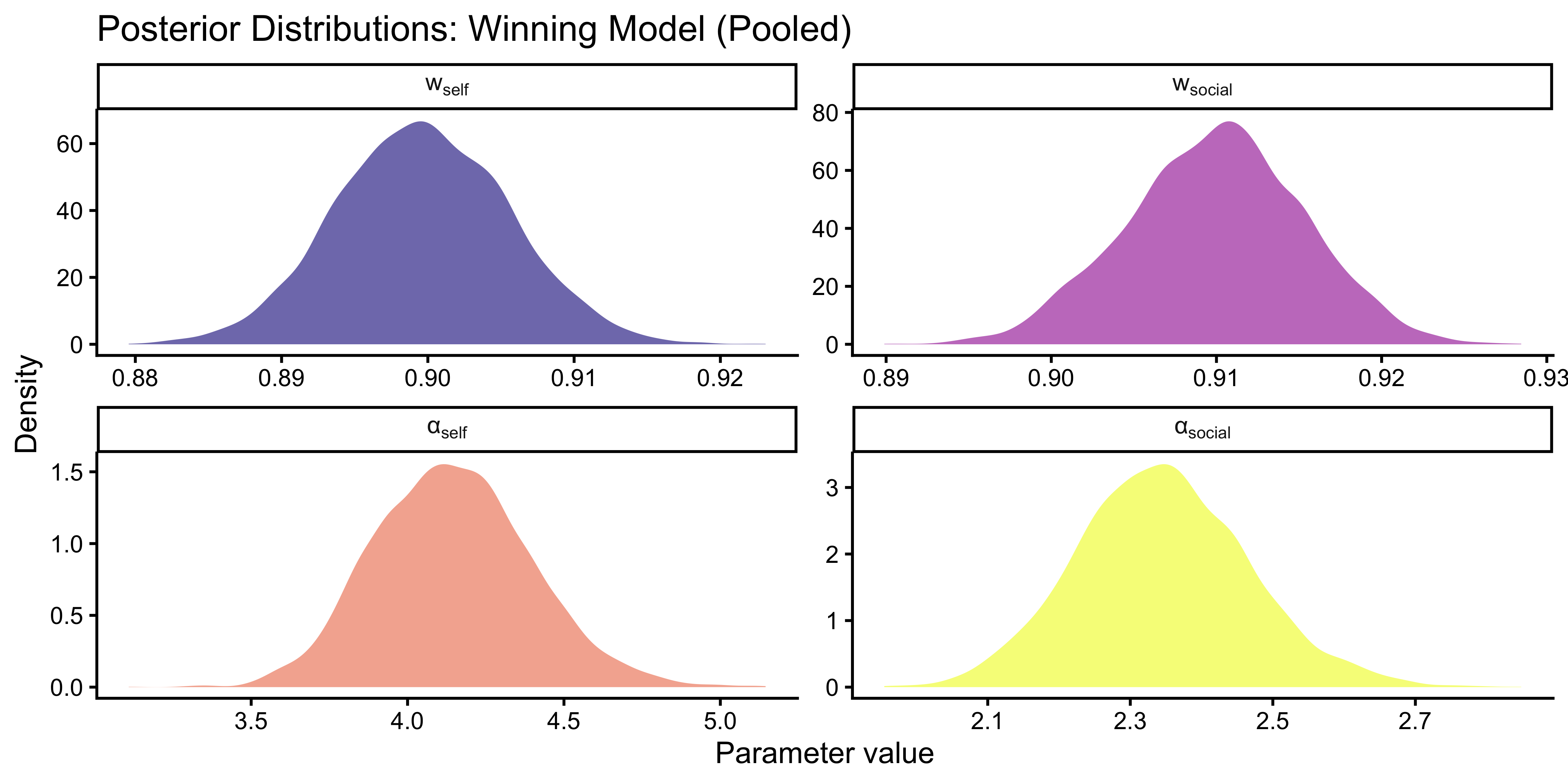
## Interpreting the Winning Model
### Parameter Posteriors (Pooled Sample)
```{r ch11b_params_pooled}
# Print posterior summary for the winning model
best_fit$summary(c("w_self", "w_social",
                   "alpha_self_m1", "alpha_social_m1",
                   "alpha_self", "alpha_social"))
```
```{r ch11b_params_pooled_plot, fig.height=4}
params_df <- best_fit$draws(
  c("w_self", "w_social", "alpha_self", "alpha_social"),
  format = "df"
) |>
  pivot_longer(c(w_self, w_social, alpha_self, alpha_social),
               names_to = "parameter", values_to = "value") |>
  mutate(parameter = factor(parameter,
    levels = c("w_self", "w_social", "alpha_self", "alpha_social"),
    labels = c("w[self]", "w[social]", "α[self]", "α[social]")))

ggplot(params_df, aes(x = value, fill = parameter)) +
  geom_density(alpha = 0.6, colour = NA) +
  facet_wrap(~parameter, scales = "free", labeller = label_parsed) +
  scale_fill_viridis_d(option = "plasma", guide = "none") +
  labs(
    title = "Posterior Distributions: Winning Model (Pooled)",
    x = "Parameter value", y = "Density"
  )
```
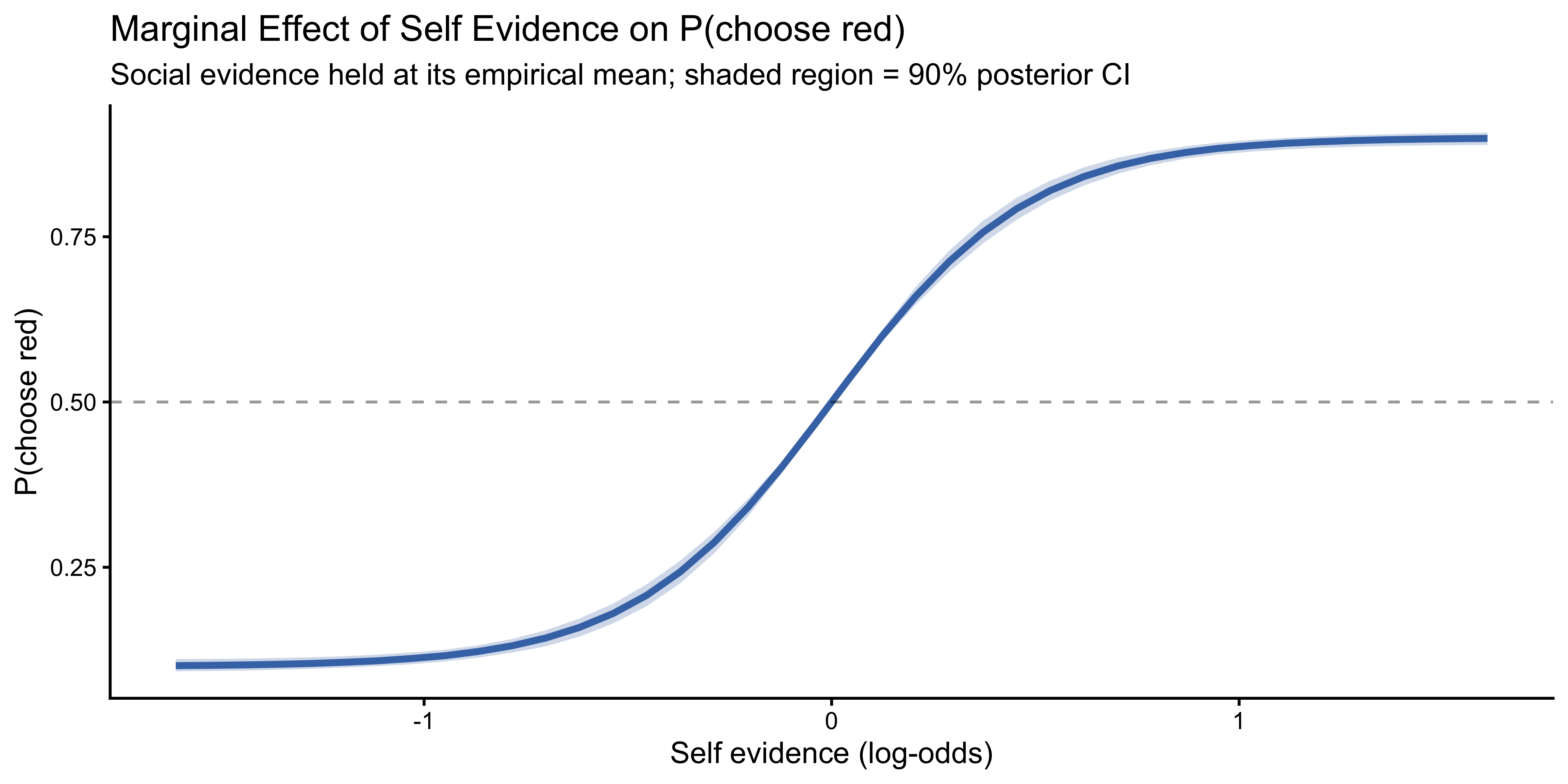
### Marginal Effects
The non-linearity of the Jardri function means that the effect of self evidence on P(choose red) depends on both the current evidence level and the model parameters. We compute **average marginal effects** by holding social evidence at its mean log-odds and varying self evidence across its observed range, using the full posterior:
```{r ch11b_marginal_effects, fig.height=4}
# Draw posterior samples
post_df <- best_fit$draws(
  c("w_self", "w_social", "alpha_self", "alpha_social"),
  format = "df"
) |>
  slice_sample(n = 500)

lo_social_mean <- mean(df$lo_social)
lo_self_grid   <- seq(min(df$lo_self), max(df$lo_self), length.out = 40)

# For CI-Loops model: L_post = jardri_f(a_s*lo_s, w_s) + jardri_f(a_o*lo_o_mean, w_o)
me_df <- map_dfr(seq_len(nrow(post_df)), function(r) {
  ws <- post_df$w_self[r]
  wo <- post_df$w_social[r]
  # Handle models with or without alpha
  if ("alpha_self" %in% names(post_df)) {
    as_ <- post_df$alpha_self[r]
    ao_ <- post_df$alpha_social[r]
    p_red <- plogis(
      jardri_f(as_ * lo_self_grid, ws) +
      jardri_f(ao_ * lo_social_mean, wo)
    )
  } else {
    p_red <- plogis(
      jardri_f(lo_self_grid, ws) +
      jardri_f(lo_social_mean, wo)
    )
  }
  tibble(lo_self = lo_self_grid, p_red = p_red, draw = r)
}) |>
  group_by(lo_self) |>
  summarise(
    lo = quantile(p_red, 0.05),
    hi = quantile(p_red, 0.95),
    med = median(p_red),
    .groups = "drop"
  )

ggplot(me_df, aes(x = lo_self)) +
  geom_ribbon(aes(ymin = lo, ymax = hi), alpha = 0.25, fill = "#4575b4") +
  geom_line(aes(y = med), colour = "#4575b4", linewidth = 1.2) +
  geom_hline(yintercept = 0.5, linetype = "dashed", alpha = 0.4) +
  labs(
    title    = "Marginal Effect of Self Evidence on P(choose red)",
    subtitle = "Social evidence held at its empirical mean; shaded region = 90% posterior CI",
    x        = "Self evidence (log-odds)",
    y        = "P(choose red)"
  )
```
## Group Differences: Controls vs Schizophrenia
### Separate Fits by Group
We now fit the winning model separately to each group. This allows direct comparison of the weight and loop parameters between healthy controls and patients with schizophrenia.
```{r ch11b_fit_by_group}
make_stan_data_lo <- function(grp) {
  d <- df |> filter(group_label == grp)
  list(
    N        = nrow(d),
    y        = d$choice_red,
    k_self   = d$k_self,   n_self   = d$n_self,
    k_social = d$k_social, n_social = d$n_social,
    run_diagnostics = 1L
  )
}

if (regenerate_fits || !file.exists("simmodels/ch11b_ctrl_fit.rds")) {

  fit_ctrl <- mod_ci_lo$sample(
    data = make_stan_data_lo("Control"),
    chains = 4, parallel_chains = 4,
    iter_warmup = 1000, iter_sampling = 1000, refresh = 0
  )

  fit_scz <- mod_ci_lo$sample(
    data = make_stan_data_lo("Schizophrenia"),
    chains = 4, parallel_chains = 4,
    iter_warmup = 1000, iter_sampling = 1000, refresh = 0
  )

  fit_ctrl$save_object("simmodels/ch11b_ctrl_fit.rds")
  fit_scz$save_object("simmodels/ch11b_scz_fit.rds")

} else {
  fit_ctrl <- readRDS("simmodels/ch11b_ctrl_fit.rds")
  fit_scz  <- readRDS("simmodels/ch11b_scz_fit.rds")
}
```
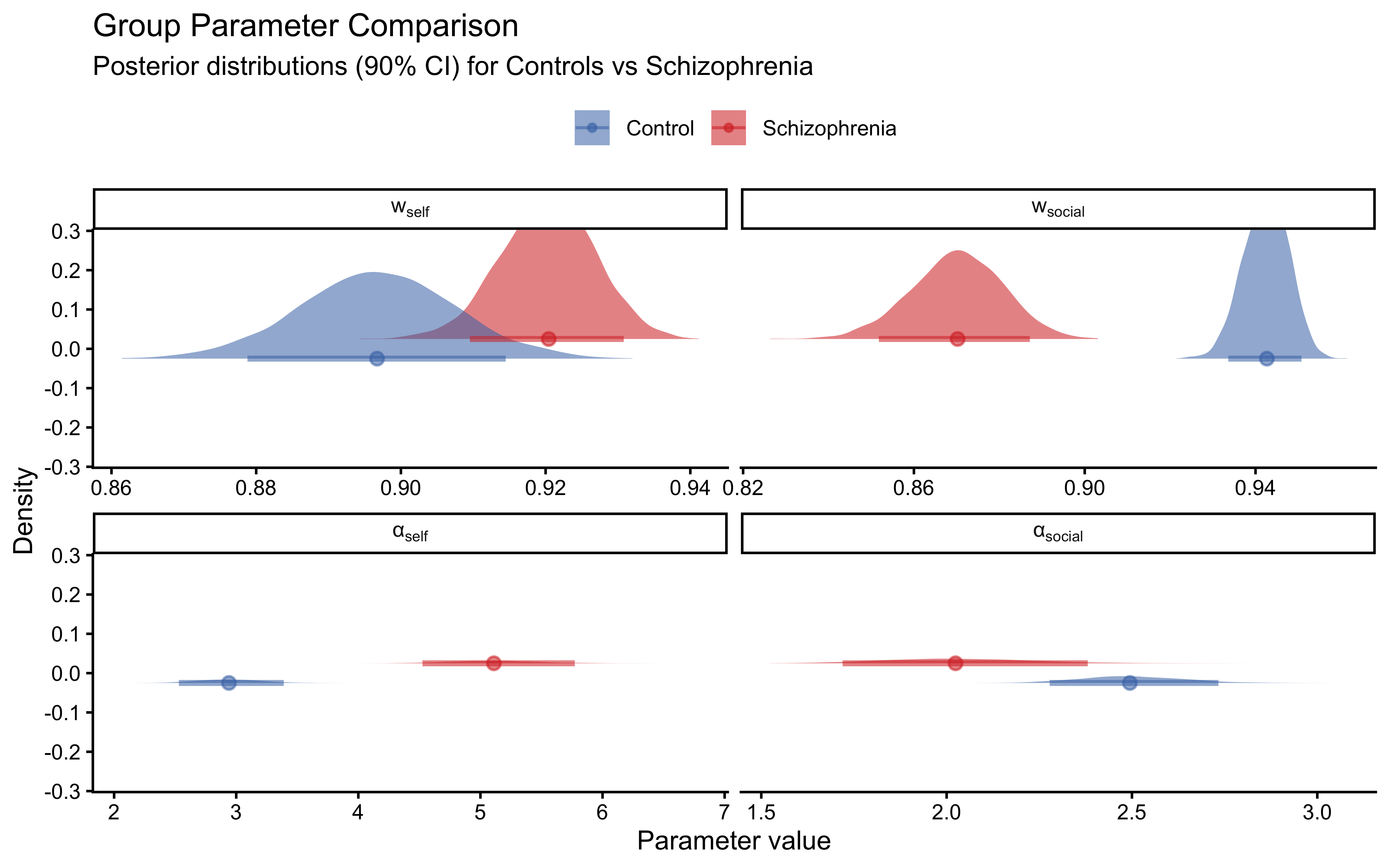
### Comparing Parameter Posteriors
```{r ch11b_group_params}
extract_params <- function(fit, grp) {
  fit$draws(c("w_self", "w_social", "alpha_self", "alpha_social"),
             format = "df") |>
    pivot_longer(c(w_self, w_social, alpha_self, alpha_social),
                 names_to = "parameter", values_to = "value") |>
    mutate(group = grp)
}

group_params <- bind_rows(
  extract_params(fit_ctrl, "Control"),
  extract_params(fit_scz,  "Schizophrenia")
) |>
  mutate(
    parameter = factor(parameter,
      levels = c("w_self", "w_social", "alpha_self", "alpha_social"),
      labels = c("w[self]", "w[social]", "α[self]", "α[social]"))
  )

ggplot(group_params, aes(x = value, fill = group, colour = group)) +
  stat_halfeye(alpha = 0.55, .width = 0.90, point_interval = "median_qi",
               position = position_dodge(width = 0.1)) +
  facet_wrap(~parameter, scales = "free_x", labeller = label_parsed) +
  scale_fill_manual(values   = pal_group) +
  scale_colour_manual(values = pal_group) +
  labs(
    title    = "Group Parameter Comparison",
    subtitle = "Posterior distributions (90% CI) for Controls vs Schizophrenia",
    x = "Parameter value", y = "Density", fill = NULL, colour = NULL
  ) +
  theme(legend.position = "top")
```
```{r ch11b_group_summary}
bind_rows(
  fit_ctrl$summary(c("w_self", "w_social", "alpha_self", "alpha_social")) |>
    mutate(group = "Control"),
  fit_scz$summary(c("w_self", "w_social", "alpha_self", "alpha_social")) |>
    mutate(group = "Schizophrenia")
) |>
  dplyr::select(group, variable, median, q5, q95) |>
  arrange(variable, group)
```
### Posterior Contrast
To quantify the group difference formally, we compute the posterior probability that patients have a higher loop parameter for self evidence than controls:
```{r ch11b_group_contrast}
ctrl_a_self <- fit_ctrl$draws("alpha_self", format = "df")$alpha_self
scz_a_self  <- fit_scz$draws("alpha_self",  format = "df")$alpha_self

# Align sample lengths
n_min <- min(length(ctrl_a_self), length(scz_a_self))
cat("P(α_self[SCZ] > α_self[CTRL]):",
    round(mean(scz_a_self[1:n_min] > ctrl_a_self[1:n_min]), 3), "\n")
ctrl_w_soc <- fit_ctrl$draws("w_social", format = "df")$w_social
scz_w_soc  <- fit_scz$draws("w_social",  format = "df")$w_social
cat("P(w_social[CTRL] > w_social[SCZ]):",
    round(mean(ctrl_w_soc[1:n_min] > scz_w_soc[1:n_min]), 3), "\n")
```
### Group Psychometric Curves from Winning Model
```{r ch11b_group_psychometric, fig.height=5}
predict_group <- function(fit_obj, grp_label) {
  post <- fit_obj$draws(c("w_self", "w_social", "alpha_self", "alpha_social"),
                         format = "df") |>
    slice_sample(n = 200)
  lo_soc_mean <- df |> filter(group_label == grp_label) |>
                   pull(lo_social) |> mean()
  lo_self_grid <- seq(-2, 2, length.out = 30)

  map_dfr(seq_len(nrow(post)), function(r) {
    tibble(
      lo_self   = lo_self_grid,
      p_red     = plogis(jardri_f(post$alpha_self[r]   * lo_self_grid, post$w_self[r]) +
                         jardri_f(post$alpha_social[r] * lo_soc_mean,  post$w_social[r])),
      draw = r, group = grp_label
    )
  }) |>
  group_by(lo_self, group) |>
  summarise(lo = quantile(p_red, 0.05), hi = quantile(p_red, 0.95),
            med = median(p_red), .groups = "drop")
}

pred_groups <- bind_rows(
  predict_group(fit_ctrl, "Control"),
  predict_group(fit_scz,  "Schizophrenia")
)

ggplot(pred_groups, aes(x = lo_self, fill = group, colour = group)) +
  geom_ribbon(aes(ymin = lo, ymax = hi), alpha = 0.25, colour = NA) +
  geom_line(aes(y = med), linewidth = 1.2) +
  geom_hline(yintercept = 0.5, linetype = "dashed", alpha = 0.4) +
  scale_fill_manual(values = pal_group) +
  scale_colour_manual(values = pal_group) +
  labs(
    title    = "Predicted Psychometric Curves by Group",
    subtitle = "Social evidence at group mean; ribbon = 90% posterior CI",
    x        = "Self evidence (log-odds)",
    y        = "P(choose red)",
    fill = NULL, colour = NULL
  ) +
  theme(legend.position = "top")
```
## Summary and Interpretation
The analyses in this chapter converge on three conclusions:
**1. Pseudo-count models capture the main effect of evidence but cannot explain the extremes.** The SBA, PBA, and WBA each fit the central part of the psychometric curves reasonably well, but the Beta-Binomial data model's probability-matching assumption is too variable at the tails: it underestimates how often participants are confidently correct when evidence is near-unanimous. LOO comparison favours the reparameterised WBA over the SBA, confirming that self and social evidence are not counted symmetrically.
**2. Among log-odds models, Weighted Bayes and Circular Inference without Interference are competitive.** The Simple Bayes model (equal face-value weighting) fits substantially worse — evidence is not taken at face value. Adding weights improves fit; adding loop parameters provides a further gain in ELPD. The interference term provides marginal additional improvement, consistent with the original Simonsen et al. findings.
**3. The two groups differ in their weight and loop parameters in the theoretically predicted direction.** Controls show higher social weight ($w_\text{social}$) and lower self-loop parameter ($\alpha_\text{self}$) than patients with schizophrenia. Patients' elevated $\alpha_\text{self}$ means they effectively amplify their own perceptual evidence, fitting the clinical picture of self-referential thinking and reduced responsiveness to disconfirming social input. This quantitative signature — the loop parameter — provides a computational marker of a core symptom dimension in schizophrenia.
### Limitations
1. **Pooled analysis ignores individual differences.** The fits in this chapter treat all participants within a group as exchangeable. A hierarchical (multilevel) extension — following Chapter 11's framework — would partial out individual variation and provide more reliable group-level estimates. The current estimates are biased toward average behaviour and may inflate uncertainty at the group level.
2. **Response time is unused.** The dataset includes reaction times (`RT`). A joint model of choices and RTs (e.g., a drift-diffusion extension) could separate decision confidence from evidence accumulation rate, potentially disentangling the weights from the loop parameters.
3. **The observation model is fixed.** All log-odds models use a Bernoulli data model (logistic link). A softmax model with a free inverse temperature would test whether participants' response determinism differs between groups, which is a separate cognitive dimension from evidence weighting.
## Further Reading
- Jardri, R., & Denève, S. (2013). Circular inferences in schizophrenia. *Brain*, 136(11), 3227–3241.
- Simonsen, A., et al. (2021). Computationally defined markers of uncertainty in the theory of mind predict the severity of clinical symptoms in schizophrenia. *Schizophrenia Bulletin*, 47(6), 1704–1714.
- Corlett, P. R., Frith, C. D., & Fletcher, P. C. (2009). From drugs to deprivation: A Bayesian framework for understanding models of psychosis. *Psychopharmacology*, 206(4), 515–530.
- Adams, R. A., Stephan, K. E., Brown, H. R., Frith, C. D., & Friston, K. J. (2013). The computational anatomy of psychosis. *Frontiers in Psychiatry*, 4, 47.