# Categorization Models: Prototypes
```{r ch13_setup, include=FALSE}
knitr::opts_chunk$set(
echo = TRUE,
warning = FALSE,
message = FALSE,
fig.width = 8,
fig.height = 5,
fig.align = "center",
out.width = "80%",
dpi = 300
)
# Set to TRUE to rerun all Stan fits and heavy simulations; FALSE loads saved results.
regenerate_simulations <- FALSE
# Set to TRUE to run the long-running validation chunks
# (LFO-CV, precision analysis, SBC). FALSE loads cached results
# or skips the chunk if no cache exists.
run_intensive_checks <- regenerate_simulations
pacman::p_load(
tidyverse, # data manipulation and visualization
here, # robust project-relative paths
mvtnorm, # multivariate normal densities
patchwork, # combining plots
cmdstanr, # Stan interface
posterior, # tidy posterior arrays
tidybayes, # tidy extraction of draws
bayesplot, # MCMC diagnostic plots
loo, # LOO-CV and PSIS
SBC, # Simulation-Based Calibration Checks
priorsense, # prior sensitivity
future, # parallel processing
furrr, # parallel functional programming
ellipse, # uncertainty ellipses
matrixStats, # logSumExp for the LFO-CV implementation
MASS, # ginv (pseudo-inverse fallback)
gridExtra,
hexbin,
magick
)
theme_set(theme_classic())
# Prior hyperparameters for log(r) and log(q)
LOG_R_PRIOR_MEAN <- 0 # prior median r = 1
LOG_R_PRIOR_SD <- 1.0 # covers r ≈ 0.13–7.4 at ±2 SD
LOG_Q_PRIOR_MEAN <- -2 # prior median q ≈ 0.14 (small drift)
LOG_Q_PRIOR_SD <- 1.0 # covers q ≈ 0.02–1.0 at ±2 SD
for (d in c("stan", "simdata", "simmodels")) {
if (!dir.exists(d)) dir.create(d)
}
# ── Shared diagnostic helper (canonical version lives in Ch 11) ──────────────
# We re-define it here for standalone use. The function returns a one-row
# tibble summarising the mandatory MCMC diagnostic battery for a cmdstanr
# fit, and prints a warning if any threshold is breached. Chapters 11, 12,
# 13, and 15 all call this so the diagnostic table looks the same everywhere.
diagnostic_summary_table <- function(fit, params = NULL) {
diag <- fit$diagnostic_summary(quiet = TRUE)
draws_summary <- fit$summary(variables = params)
# Calculate individual metrics
n_div <- sum(diag$num_divergent)
max_rhat <- round(max(draws_summary$rhat, na.rm = TRUE), 2)
min_bulk <- round(min(draws_summary$ess_bulk, na.rm = TRUE), 0)
min_tail <- round(min(draws_summary$ess_tail, na.rm = TRUE), 0)
min_ebfmi <- round(min(diag$ebfmi), 3)
# Robust MCSE calculation
mcse_col <- intersect(names(draws_summary), c("mcse_mean", "mcse", "mcse_cp"))[1]
if (!is.na(mcse_col)) {
max_mcse <- round(max(draws_summary[[mcse_col]] / draws_summary$sd, na.rm = TRUE), 4)
} else {
max_mcse <- round(max(1 / sqrt(draws_summary$ess_bulk), na.rm = TRUE), 4)
}
# Build the formatted table
out <- tibble::tibble(
metric = c(
"Divergences (zero tolerance)",
"Max rank-normalised R-hat",
"Min bulk ESS",
"Min tail ESS",
"Min E-BFMI",
"Max MCSE / posterior SD"
),
value = c(n_div, max_rhat, min_bulk, min_tail, min_ebfmi, max_mcse),
threshold = c("== 0", "< 1.01", "> 400", "> 400", "> 0.2", "< 0.05"),
pass = c(
n_div == 0,
max_rhat < 1.01,
min_bulk > 400,
min_tail > 400,
min_ebfmi > 0.2,
max_mcse < 0.05
)
)
# Check if any threshold failed
if (!all(out$pass)) {
warning(
"MCMC diagnostic battery: at least one threshold breached. ",
"Inspect divergences and reparameterize before interpreting the posterior.",
call. = FALSE
)
}
out
}
# ── Kruschke (1993) stimulus set ─────────────────────────────────────────────
# Re-defined here for standalone use; identical to Ch. 11.
stimulus_info <- tibble(
stimulus = c(5, 3, 7, 1, 8, 2, 6, 4),
height = c(1, 1, 2, 2, 3, 3, 4, 4),
position = c(2, 3, 1, 4, 1, 4, 2, 3),
category_true = c(0, 0, 1, 0, 1, 0, 1, 1)
)
n_blocks <- 8
n_stim_per_block <- nrow(stimulus_info)
total_trials <- n_blocks * n_stim_per_block
# ── Per-subject schedule helper ───────────────────────────────────────────────
# Identical to Ch. 11. Redefined here for standalone use.
make_subject_schedule <- function(stimulus_info, n_blocks, seed) {
set.seed(seed)
n_stim <- nrow(stimulus_info)
sequence <- unlist(lapply(seq_len(n_blocks), function(b) {
sample(stimulus_info$stimulus, n_stim, replace = FALSE)
}))
tibble(
trial_within_subject = seq_along(sequence),
block = rep(seq_len(n_blocks), each = n_stim),
stimulus_id = sequence
) |>
left_join(stimulus_info, by = c("stimulus_id" = "stimulus")) |>
rename(category_feedback = category_true) |>
dplyr::select(trial_within_subject, block, stimulus_id,
height, position, category_feedback)
}
plan(multisession, workers = max(1, availableCores() - 1))
```
> **📍 Where we are in the Bayesian modeling workflow:**
> Chapter 13 built the GCM — an exemplar model that stores every encountered
> stimulus and decides by summed similarity to memory. This chapter introduces
> a structurally different account: the **prototype model**, which abstracts
> each category to a single running estimate (its mean and uncertainty) rather
> than storing individual instances. We implement prototype learning as a
> multivariate Kalman filter and then add a **Stan parameter-estimation model**
> for the prototype architecture.
>
> The full validation pipeline from Ch. 5 — prior
> predictive check, Pathfinder initialization, mandatory MCMC diagnostic
> battery, posterior predictive check, prior–posterior update plot, randomised
> LOO-PIT, LFO-CV, precision analysis, prior sensitivity,
> and SBC — is applied to this new model. Crucially, the **LFO-CV machinery
> implemented in Chapter 13** (`psis_lfo_gcm`) is generalised here as
> `psis_lfo_kalman` and applied to the prototype model. The chapter then
> extends to a **multilevel prototype model** with population-level priors
> on `log_r`, per-subject NCP offsets, and the full multilevel SBC battery
> (population and individual calibration).
## Rethinking Category Representation: From Examples to Averages
In the previous chapter, we explored the Generalized Context Model (GCM), an exemplar model where every encountered example is stored in memory. This approach is powerful but raises questions about cognitive efficiency. Do we really store every single instance we encounter?
Consider learning about common categories like "birds" or "chairs". While specific examples matter, we also seem to develop a general sense of what constitutes a typical member. Prototype theory offers an alternative perspective: instead of storing individual exemplars, the mind abstracts a summary representation — a prototype — for each category. This prototype often represents the central tendency or "average" member.
## Core Ideas of Prototype Models
| Feature | Prototype Models | Exemplar Models (GCM) |
|---|---|---|
| Representation | Abstract summary (e.g., average) | Collection of individual examples |
| Memory Cost | Low (one prototype per category) | High (potentially all examples) |
| Key Information | Central tendency & variance | Specific instances & their labels |
| Sensitivity | Less sensitive to specific examples | Highly sensitive to specific examples |
::: {.callout-note}
### Historical Context: From Typicality Effects to Dynamic Prototypes
The prototype approach to categorization did not emerge fully formed. It arose as the solution to a specific failure mode of the dominant view (rules) and evolved in a debate with alternative approaches (exemplars).
#### The Classical View and Its Discontents
Through the 1950s and into the 1960s, both philosophers and psychologists took it for granted that concepts had *defining features*: necessary and sufficient conditions that every member must satisfy. A bachelor is an unmarried adult male — full stop. Categorization, on this view, was logical: check the features, apply the rule. The model is appealingly crisp, but Wittgenstein had already noted the trouble in *Philosophical Investigations* (1953): most ordinary categories — *game*, *furniture*, *bird* — resist such definitions. Family resemblance, not shared essence, seemed to be the operative structure.
The empirical broadside came from Eleanor Rosch [@rosch1973natural; @rosch1975cognitive; @rosch1976basic]. In a series of influential experiments she documented **typicality effects**: robins are judged faster and more confidently as birds than penguins are; desk chairs are more chair-like than beanbags. Categories showed graded membership rather than all-or-nothing inclusion. Rosch also identified a privileged **basic level** — the level of abstraction (dog, not animal and not poodle) at which objects are most efficiently perceived, named, and remembered. Neither observation is compatible with the classical view, which predicts uniform membership within a category and no principled distinction across levels.
#### The Prototype as Psychological Mechanism
Rosch's work raised the question of *representation*: if not a rule, what mental structure supports graded membership? The answer on offer was a **prototype** — a summary representation encoding the central tendency of encountered category members. New objects are categorized by their distance from stored prototypes; items close to the prototype are typical, items distant are atypical.
Formal prototype models predated Rosch's program. @posner1968genesis showed that subjects who had studied distorted dot patterns without ever seeing the prototype nonetheless recognized the prototype at the end as highly familiar — abstraction was occurring implicitly. @reed1972pattern implemented an explicit prototype-matching classifier and showed it outperformed several alternatives on face-classification data. These early models computed a **static average** from training examples: the prototype was fixed after learning and then used as a lookup.
#### Static Prototypes and the Exemplar Challenge
The clean elegance of static prototype models made them obvious targets for empirical attack. @medin1978context showed that, on certain category structures, the Context Model (a pure exemplar model) fit human data significantly better than a prototype model could. The critical cases were **exception items**: an atypical member of one category that closely resembles the other category's prototype. Exemplar models accommodate exceptions naturally — the deviant item is stored individually. A static prototype, by definition, assimilates the deviant item into the average, smoothing away the very information that drives behavior.
Through the 1980s and early 1990s, the prototype-versus-exemplar debate generated substantial empirical literature. The consensus, codified in @smith1998prototype, was that neither account was universally superior: prototype-like effects dominated in some conditions (large training sets, brief study times, transfer to novel stimuli) while exemplar-like effects dominated in others (small training sets, extended learning, highly distinctive items). The field was left with a theoretical draw that demanded either a hybrid architecture or a shift in the question being asked.
#### From Static Averaging to Bayesian Updating
We do not take a stance here on the prototype-versus-exemplar debate. The previous chapter implemented exemplar models in some detail; this chapter sticks with prototype representations precisely so we can understand them on their own terms: what changes when the summary representation is allowed to update incrementally, how its parameters are recovered, and how it behaves under different learning environments.
Within that scope, the focus shifts from *what is stored* to *how the stored summary is updated*. A static average treats all observed members the same regardless of when they were encountered, and provides no mechanism for tracking categories that drift over time: the clothing you learn is "fashionable" today may not be fashionable in five years. Several incremental prototype schemes have been proposed in response. The simplest is a **delta rule**: $\mu_{t} = \mu_{t-1} + \alpha\,(x_t - \mu_{t-1})$, with a fixed learning rate $\alpha$ that yields exponentially weighted recency [@gluck1988conditioning; @estes1994classification]. You should recognize this rule from reinforcement learning :-) @anderson1991adaptive's rational model takes a fully Bayesian route, but over a Dirichlet-process partition rather than a parametric prototype. Each captures part of the picture: the delta rule is principled in form but its $\alpha$ is a free knob disconnected from the learner's uncertainty as it faces the stimuli; Anderson's model is Bayesian but solves a different problem (discovering the partition) and is harder to fit at the trial level.
The Kalman filter [@kalman1960new], developed originally for aerospace navigation, sits [I think, nobody else has used it for this!] in a useful intermediate position for prototype modelling. It is the **minimum-variance unbiased estimator** for a linear-Gaussian dynamical system: at each step it computes exactly how much weight to place on the new observation versus the accumulated prior, using the relative magnitudes of measurement noise $R$ and process noise $Q$. The learning rate (the Kalman gain) is not a free parameter but is *derived* at each trial from current uncertainty — recovering a delta-rule-like update whose effective $\alpha$ shrinks as evidence accumulates and grows again when the world is assumed to drift. When $Q = 0$ the prototype is assumed static and the gain decays monotonically — recovering the classical static average as a special case. When $Q > 0$ the prototype can drift and the steady-state gain remains positive, allowing perpetual sensitivity to new observations.
Applications of Kalman-style updating to human learning appear across multiple domains: classical conditioning [@dayan2000learning], interval timing, and reward prediction. The two-parameter family $(r, q)$ instantiates a spectrum from steep, responsive updating ($r$ small, gain high) to heavily smoothed abstraction ($r$ large, gain low, slow forgetting), with $q$ controlling whether the steady-state gain decays to zero or saturates above it.
#### The Bayesian Connection
Importantly for us [well, let's be honest, for me, but I'll take you along for the ride], the Kalman filter is a conceptually Bayesian method: it is the exact Bayesian posterior for a Gaussian state-space model. The prototype at trial $t$ is the posterior mean $\mathbb{E}[\mu_t \mid x_{1:t}]$; the covariance $\Sigma_t$ is the posterior variance. Recognising this identity connects the prototype model to the broader programme of **rational analysis** [@anderson1991adaptive] and **Bayesian models of cognition** [@tenenbaum2011grow]: the learner is performing optimal inference about a latent category structure given noisy, sequentially arriving evidence. The parameters $r$ and $q$ then carry clear psychological interpretations — observation noise (how variable are category members around the prototype?) and process noise (how rapidly does the category itself change?) — rather than being purely phenomenological fitting coefficients.
This framing also clarifies the key difference from the GCM: where the GCM stores the full history and retrieves it at decision time, the Kalman prototype model **compresses** the history into sufficient statistics (mean and covariance) that are updated recursively. The compression is lossless when the generative model is Gaussian and linear — which is why recovery and SBC are cleaner here than in most cognitive models of comparable scope.
:::
## Modeling Dynamic Prototypes: The Kalman Filter
Early prototype models often calculated a static average. However, human learning is dynamic; our understanding evolves with experience. How can we model a prototype that updates incrementally as new examples are encountered?
The Kalman filter provides a suitable mathematical framework. Originally developed for tracking physical systems amidst noise, it's well-suited for modeling prototype learning because it allows us to:
* **Track an Estimate**: The category prototype (its average feature values).
* **Represent Uncertainty**: Maintain not just the prototype's location but also our uncertainty about it.
* **Update Incrementally**: Refine the prototype with each new example.
* **Balance Old and New**: Optimally combine the current prototype (prior belief) with the new example (evidence).
* **Implement an Adaptive Learning Rate**: Automatically adjust how much influence a new example has (the "Kalman gain") based on current uncertainty. Learning is faster when uncertainty is high and slows as confidence grows.
### The Kalman Filter Logic: Updating an Estimate
Imagine tracking a prototype based on a single feature (e.g., average height). The Kalman filter maintains your Current State. At any moment, you have two key pieces of information:
* **Your Best Guess ($\mu$):** This is your current estimate of the prototype's average height.
* **Your Confidence ($\sigma^2$):** This isn't just *if* you're confident, but *how much*. It's the *variance* around your guess. A small variance means you're quite sure; a large variance means you're very unsure.
When a new category member (observation $x$) arrives, you measure its height.
* **The Catch:** Your measurement tool (or the example itself) isn't perfect. There's some inherent "noise" or variability in how examples relate to the true prototype. We represent the uncertainty of this *measurement process* with another variance, often called $R$.
**The Core Problem:** You have your guess (with $\sigma^2_{prev}$) and a new measurement (with $R$). How do you combine them to get a *new, better guess* and an *updated level of uncertainty*?
**Enter the Kalman Gain ($K$): The "Trust" Knob**
The Kalman filter calculates the Kalman Gain $K$, which tells you how much to trust the *new measurement* compared to your *current guess*:
$$K = \frac{\sigma^2_{prev}}{\sigma^2_{prev} + R}$$
If $\sigma^2_{prev}$ is large relative to $R$, then $K \to 1$: trust the measurement almost completely. If $\sigma^2_{prev}$ is small relative to $R$, then $K \to 0$: stick closer to your previous guess.
**Updating Your Guess:**
You nudge your old guess towards the new measurement. The size of the nudge is determined by the Kalman Gain $K$:
$$\mu_{new} = \mu_{prev} + K \cdot (x - \mu_{prev})$$
The term $(x - \mu_{prev})$ is the "prediction error" or "innovation" — how much the new data differs from what you expected.
**Updating Your Confidence (Uncertainty):**
After incorporating new information, uncertainty decreases:
$$\sigma^2_{new} = (1 - K) \cdot \sigma^2_{prev}$$
Since $K \in (0, 1)$, multiplying by $(1 - K)$ always shrinks uncertainty. The more you trusted the measurement (higher $K$), the more your uncertainty shrinks.
**Extending to drifting targets.** The scalar Kalman filter above assumes a static target: uncertainty monotonically decreases because there is no mechanism for it to grow back. The prototype model in this chapter adds a **process noise term** $Q$. Before each measurement update, a *prediction step* is applied:
$$\sigma^2_{k|k-1} = \sigma^2_{k-1|k-1} + Q$$
This increases uncertainty between observations, reflecting the possibility that the true prototype has shifted since the last trial. The subsequent measurement update then decreases uncertainty via the Kalman gain, exactly as before. At steady state, the two forces balance and uncertainty converges to a fixed value rather than shrinking to zero. When $Q = 0$ the model reduces to the static-target filter. We treat the scalar $q$ (the diagonal of $Q = q \cdot I$) as a free parameter to be estimated from data, alongside the observation noise $r$.
### Extending to Multiple Features: Multivariate Kalman Filter
Our stimuli have two features (height and position). We need a multivariate version:
* **Your Current State (Vectors and Matrices):**
* **Your Best Guess ($\vec{\mu}$):** Now a *vector* containing your best guess for each feature.
* **Your Confidence ($\Sigma$):** Now a *covariance matrix*. The diagonal elements give the variance for each feature individually; the off-diagonal elements give their covariance — for example, whether taller prototypes are also typically further to the right.
* **A New Hint Arrives:** Your new observation ($\vec{x}$) is also a vector.
* **Measurement Noise ($R$):** Also a covariance matrix. Often simplified to a diagonal matrix, assuming measurement errors on different features are independent.
* **The Logic Stays the Same, the Math Uses Matrices:**
* **Kalman Gain ($K$):** A *matrix*: $K = \Sigma_{prev} (\Sigma_{prev} + R)^{-1}$
* **Updating Your Guess ($\vec{\mu}$):** $\vec{\mu}_{new} = \vec{\mu}_{prev} + K (\vec{x} - \vec{\mu}_{prev})$
* **Updating Your Confidence ($\Sigma$):** The intuition is the same as the scalar case — uncertainty shrinks after each observation — but now in matrix form. The textbook update is $\Sigma_{new} = (I - K)\Sigma_{prev}$, which can be read as: "keep the share of the prior uncertainty that the new observation did *not* explain away." In code, however, we use the algebraically equivalent Joseph form, $\Sigma_{new} = (I - K)\Sigma_{prev}(I - K)^T + KRK^T$. This longer expression makes the two sources of remaining uncertainty explicit: the leftover prior uncertainty (first term) plus the measurement noise that leaks in through the Kalman gain (second term). The reason for using it in practice is purely numerical: a covariance matrix must be symmetric and have non-negative variances, and the Joseph form preserves both properties even when small rounding errors accumulate over many trials, whereas the shorter form can drift into invalid (asymmetric or negative-variance) territory.
### In a Nutshell
The Kalman filter tracks a prototype as a running estimate $\vec{\mu}$ and a covariance $\Sigma$ that quantifies how confident the learner is. Each trial has two phases: a *predict* step that inflates $\Sigma$ by $Q$ to allow the prototype to drift between observations, and an *update* step that pulls $\vec{\mu}$ toward the new exemplar by an amount set by the Kalman gain $K$ — high when the learner is uncertain or measurements are precise, low when the learner is already confident or measurements are noisy. The gain also determines how much $\Sigma$ shrinks. At steady state, drift ($Q$) and shrinkage balance, so uncertainty stops collapsing to zero and the model keeps learning indefinitely.
### Implementing the Multivariate Update in R
```{r ch13_multivariate_kalman_update}
# One update step of a multivariate Kalman filter.
# Returns updated mean vector, covariance matrix, and Kalman gain.
multivariate_kalman_update <- function(mu_prev,      # previous mean vector
                                       sigma_prev,    # previous covariance matrix
                                       observation,   # observed feature vector
                                       r_matrix) {    # observation noise matrix
  mu_prev     <- as.numeric(mu_prev)
  observation <- as.numeric(observation)
  sigma_prev  <- as.matrix(sigma_prev)
  r_matrix    <- as.matrix(r_matrix)

  n_dim <- length(mu_prev)
  I     <- diag(n_dim)

  # Kalman gain: K = Sigma_prev * (Sigma_prev + R)^{-1}
  S     <- sigma_prev + r_matrix
  S_inv <- tryCatch(
    solve(S),
    error = function(e) {
      warning("Matrix inversion failed; using pseudo-inverse.", call. = FALSE)
      MASS::ginv(S)
    }
  )
  K <- sigma_prev %*% S_inv

  # Update mean
  innovation <- observation - mu_prev
  mu_new     <- as.numeric(mu_prev + K %*% innovation)

  # Update covariance — Joseph form for numerical stability
  IK        <- I - K
  sigma_new <- IK %*% sigma_prev %*% t(IK) + K %*% r_matrix %*% t(K)

  # Enforce symmetry (floating-point can introduce tiny asymmetry)
  sigma_new <- (sigma_new + t(sigma_new)) / 2

  list(mu = mu_new, sigma = sigma_new, k = K)
}
```
This function performs a single update for one category's prototype when it observes a new member.
---
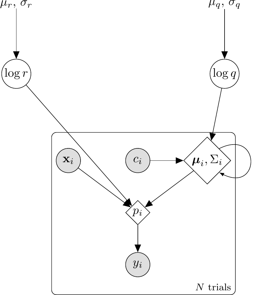
We are fitting a *two-parameter* model: $r$ controls both Kalman gain and decisional precision; $q$ controls prototype drift speed and steady-state uncertainty. Both are inferred from data on the log scale. There is no category bias, fixed initial means, fixed initial covariances, and diagonal noise structures for both $R$ and $Q$. The Stan implementation in §"The Prototype Model in Stan" implements exactly this.
```{tikz prototype-single-dag, fig.cap = "DAG for the single-subject prototype (Kalman) model. Hyperparameters (dots) feed into the two latent parameters (circles): $\\log r$ (observation noise) and $\\log q$ (process noise). Inside the trial plate, the stimulus $\\mathbf{x}_i$ and feedback $c_i$ combine with the carried-forward state $(\\boldsymbol{\\mu}_i, \\Sigma_i)$ — which is updated across trials via the Kalman predict/update steps — to yield the deterministic choice probability $p_i$ (double circle), from which the response $y_i$ is drawn. The self-loop on the state node represents the sequential prototype update.", fig.align = "center", out.width = "70%"}
\usetikzlibrary{bayesnet}
\begin{tikzpicture}
  % ── Hyperparameters (const) ─────────────────────────────
  \node[const] (hyp_r) at (0, 0) {$\mu_r,\,\sigma_r$};
  \node[const] (hyp_q) at (6, 0) {$\mu_q,\,\sigma_q$};

  % ── Latent parameters ───────────────────────────────────
  \node[latent] (logr) at (0, -2) {$\log r$};
  \node[latent] (logq) at (6, -2) {$\log q$};

  % ── Trial-level nodes (inside plate) ────────────────────
  \node[obs] (xi)    at (1.5, -4.5) {$\mathbf{x}_i$};
  \node[obs] (ci)    at (3.5, -4.5) {$c_i$};
  \node[det] (state) at (5.5, -4.5) {$\boldsymbol{\mu}_i,\Sigma_i$};
  \node[det] (pi)    at (3.5, -6.0) {$p_i$};
  \node[obs] (yi)    at (3.5, -7.5) {$y_i$};

  % ── Edges ───────────────────────────────────────────────
  \edge {hyp_r} {logr};
  \edge {hyp_q} {logq};
  \edge {logq}  {state};
  \edge {ci}    {state};
  \edge {state} {pi};
  \edge {xi}    {pi};
  \edge {logr}  {pi};
  \edge {pi}    {yi};

  % ── Self-loop on state (sequential update) ─────────────
  \draw[->, >=latex] (state.north east) .. controls +(1.2,0.6) and +(1.2,-0.6) .. (state.south east);

  % ── Plate ───────────────────────────────────────────────
  \plate {trial} {(xi)(ci)(state)(pi)(yi)} {$N$ trials};
\end{tikzpicture}
```
---
## Building the Full Categorization Model
We now integrate this update mechanism into a full agent that learns prototypes for two categories and makes categorization decisions.
### Initialization
* We need separate prototypes ($\mu_0, \Sigma_0$ and $\mu_1, \Sigma_1$) for Category 0 and Category 1.
* We start with high uncertainty (large initial $\Sigma$) and uninformative means at the center of the feature space.
* We define the observation noise matrix $R = r_\text{val} \cdot I$. The parameter $r_\text{val}$ represents how much variability we assume exists within categories or in our perception of stimuli.
* We define the process noise matrix $Q = q_\text{val} \cdot I$. The parameter $q_\text{val}$ controls how much the category prototype may drift between successive observations. Small $q$ means near-static categories; large $q$ means rapidly shifting ones.
### Categorization Decision
How does the model decide which category a new stimulus $\vec{x}$ belongs to? The decision has three steps: compute a **distance** from the stimulus to each prototype, convert distance to **similarity**, then apply a **choice rule**.
**Step 1 — Distance.** The distance between stimulus $\vec{x}$ and category $C$'s prototype is the Mahalanobis distance:
$$d_C = (\vec{x} - \vec{\mu}_C)^T (\Sigma_C + R)^{-1} (\vec{x} - \vec{\mu}_C)$$
Breaking this down for two features (height and position):
$$d_C = \frac{(x_\text{height} - \mu_{C,\text{height}})^2}{\sigma_{C,\text{height}}^2 + r} + \frac{(x_\text{position} - \mu_{C,\text{position}})^2}{\sigma_{C,\text{position}}^2 + r}$$
Each feature contributes its squared difference divided by total uncertainty on that dimension. The three quantities that enter are:
* $\vec{\mu}_C$: the prototype mean — the Kalman filter's current best estimate of the category centre.
* $\Sigma_C$: the prototype uncertainty — a matrix tracking how confident the filter is about that estimate. It starts large (high uncertainty) and shrinks as more examples are seen. High uncertainty on dimension $k$ means differences on that dimension count for less in the distance.
* $R = r \cdot I$: observation noise — a fixed matrix reflecting how variable category members are around the prototype, or how noisy perception is. Together with $\Sigma_C$, it forms the total uncertainty $\Sigma_C + R$ that normalises each squared difference.
**Step 2 — Similarity.** Distance is converted to similarity by an exponential decay:
$$\eta_C = \exp\!\left(-\tfrac{1}{2}\, d_C\right)$$
This is the multivariate normal density evaluated at $\vec{x}$. Similarity is 1 when the stimulus sits exactly on the prototype mean ($d_C = 0$) and falls toward 0 as distance grows. The parameter $r$ controls how steeply: large $r$ inflates the denominators in $d_C$, shrinks the distance, and produces a flat bell curve — the model generalises broadly. Small $r$ produces a sharp bell curve — only stimuli very close to the prototype receive high similarity. This is the role that the sensitivity parameter $c$ plays in the GCM's $\exp(-c \cdot d)$; here it is embedded inside the distance rather than sitting outside it.
**Step 3 — Choice rule.** The probability of choosing Category 1 is the proportion of total similarity belonging to that category (Luce choice rule):
$$P(\text{Choose Cat 1} \mid \vec{x}) = \frac{\eta_1}{\eta_0 + \eta_1}$$
We work with log-probabilities for numerical stability. There is no separate softmax temperature: $r$ already controls decisional sharpness through the similarity step.
### The Learning Loop
The agent processes trials sequentially:
1. **Predict**: Add $Q$ to both category covariances — $\Sigma_{0} \mathrel{+}= Q$, $\Sigma_{1} \mathrel{+}= Q$ — reflecting that each prototype may have drifted since the last observation.
2. **Decide**: Calculate $P(\text{Choose Cat 1} \mid \vec{x}_i)$ based on the post-prediction $\mu_0, \Sigma_0, \mu_1, \Sigma_1$.
3. **Respond**: Generate a response.
4. **Receive feedback**: Observe true category $y_i$.
5. **Update**: Apply the Kalman measurement update to the correct category only.
### R Implementation of the Prototype Agent
Each agent's learning trajectory depends on the order in which stimuli are encountered, and different randomizations produce genuinely different trajectories.
```{r ch13_prototype_model}
# Prototype model agent using Kalman filter with process noise for categorization.
# r_value   : observation noise variance (scalar > 0)
# q_value   : process noise variance / prototype drift rate (scalar >= 0)
# obs       : matrix of observations (trials x features)
# cat_one   : vector of true category labels (0 or 1) for feedback
# Returns:  tibble with prob_cat1 and sim_response
prototype_kalman <- function(r_value,
                             q_value,
                             obs,
                             cat_one,
                             initial_mu         = NULL,
                             initial_sigma_diag = 10.0,
                             quiet              = TRUE) {
  n_trials   <- nrow(obs)
  n_features <- ncol(obs)

  if (is.null(initial_mu)) {
    mu0_init <- rep(2.5, n_features)
    mu1_init <- rep(2.5, n_features)
  } else {
    mu0_init <- initial_mu[[1]]
    mu1_init <- initial_mu[[2]]
  }

  prototype_cat_0 <- list(mu = mu0_init, sigma = diag(initial_sigma_diag, n_features))
  prototype_cat_1 <- list(mu = mu1_init, sigma = diag(initial_sigma_diag, n_features))
  r_matrix        <- diag(r_value, n_features)
  q_matrix        <- diag(q_value, n_features)

  response_probs <- numeric(n_trials)

  log_sum_exp <- function(v) {
    m <- max(v)
    m + log(sum(exp(v - m)))
  }

  for (i in seq_len(n_trials)) {
    if (!quiet && i %% 20 == 0) cat("Trial", i, "\n")

    current_obs <- as.numeric(obs[i, ])

    # ── Prediction step: add process noise to both prototypes ──────────────
    # Reflects potential drift in category location since last trial.
    # When q_value = 0 this reduces to the static-target filter.
    prototype_cat_0$sigma <- prototype_cat_0$sigma + q_matrix
    prototype_cat_1$sigma <- prototype_cat_1$sigma + q_matrix

    # ── Decision ─────────────────────────────────────────────────────────────
    cov_cat_0 <- prototype_cat_0$sigma + r_matrix
    cov_cat_1 <- prototype_cat_1$sigma + r_matrix

    log_prob_0 <- tryCatch(
      mvtnorm::dmvnorm(current_obs, mean = prototype_cat_0$mu,
                       sigma = cov_cat_0, log = TRUE),
      error = function(e) -Inf
    )
    log_prob_1 <- tryCatch(
      mvtnorm::dmvnorm(current_obs, mean = prototype_cat_1$mu,
                       sigma = cov_cat_1, log = TRUE),
      error = function(e) -Inf
    )

    if (!is.finite(log_prob_0) && !is.finite(log_prob_1)) {
      prob_cat_1 <- 0.5
    } else if (!is.finite(log_prob_0)) {
      prob_cat_1 <- 1.0
    } else if (!is.finite(log_prob_1)) {
      prob_cat_1 <- 0.0
    } else {
      prob_cat_1 <- exp(log_prob_1 - log_sum_exp(c(log_prob_0, log_prob_1)))
    }
    response_probs[i] <- pmax(1e-9, pmin(1 - 1e-9, prob_cat_1))

    # ── Update (measurement update for the correct category only) ────────────
    true_cat <- cat_one[i]
    if (true_cat == 1) {
      upd <- multivariate_kalman_update(prototype_cat_1$mu, prototype_cat_1$sigma,
                                        current_obs, r_matrix)
      prototype_cat_1$mu    <- upd$mu
      prototype_cat_1$sigma <- upd$sigma
    } else {
      upd <- multivariate_kalman_update(prototype_cat_0$mu, prototype_cat_0$sigma,
                                        current_obs, r_matrix)
      prototype_cat_0$mu    <- upd$mu
      prototype_cat_0$sigma <- upd$sigma
    }
  }

  tibble(
    prob_cat1    = response_probs,
    sim_response = rbinom(n_trials, 1, response_probs)
  )
}

# Wrapper: generates per-agent schedule then calls prototype_kalman
simulate_prototype_agent <- function(agent_id, r_value, q_value,
                                     stimulus_info, n_blocks, subject_seed) {
  schedule <- make_subject_schedule(stimulus_info, n_blocks, seed = subject_seed)
  obs      <- as.matrix(schedule[, c("height", "position")])
  cat_one  <- schedule$category_feedback

  result <- prototype_kalman(
    r_value            = r_value,
    q_value            = q_value,
    obs                = obs,
    cat_one            = cat_one,
    initial_mu         = list(rep(2.5, 2), rep(2.5, 2)),
    initial_sigma_diag = 10.0,
    quiet              = TRUE
  )

  schedule |>
    mutate(
      agent_id     = agent_id,
      r_value_true = r_value,
      q_value_true = q_value,
      log_r_true   = log(r_value),
      log_q_true   = log(q_value),
      prob_cat1    = result$prob_cat1,
      sim_response = result$sim_response,
      correct      = as.integer(category_feedback == sim_response)
    ) |>
    group_by(agent_id) |>
    mutate(performance = cumsum(correct) / row_number()) |>
    ungroup()
}
```
### Simulating Categorization Behavior
Let's simulate behavior on the Kruschke (1993) task. The key parameter here is `r_value`, the observation noise. This parameter reflects the model's assumption about how much variability exists within categories or arises from perceptual noise.
* **Low `r_value`**: The model assumes observations are precise representations of the category; each new example exerts strong influence and prototypes update rapidly.
* **High `r_value`**: The model assumes observations are noisy; learning is slower as each example has less influence, but the model generalizes more broadly.
```{r ch13_simulate_prototype_responses}
param_df <- expand_grid(
  agent_id  = 1:5,
  r_value   = c(0.5, 2.0),
  q_value   = c(0.001, 0.1, 0.5)
) |>
  mutate(subject_seed = agent_id)

sim_file <- here("simdata", "ch13_prototype_simulated_responses.csv")
if (regenerate_simulations || !file.exists(sim_file)) {
  cat("Regenerating prototype simulations...\n")
  prototype_responses <- future_pmap_dfr(
    list(
      agent_id     = param_df$agent_id,
      r_value      = param_df$r_value,
      q_value      = param_df$q_value,
      subject_seed = param_df$subject_seed
    ),
    simulate_prototype_agent,
    stimulus_info = stimulus_info,
    n_blocks      = n_blocks,
    .options = furrr_options(seed = TRUE)
  )
  write_csv(prototype_responses, sim_file)
  cat("Simulations saved.\n")
} else {
  prototype_responses <- read_csv(sim_file, show_col_types = FALSE)
  cat("Simulations loaded.\n")
}
ggplot(prototype_responses,
       aes(x = trial_within_subject, y = performance, color = factor(r_value_true))) +
  stat_summary(fun = mean, geom = "line", linewidth = 1) +
  stat_summary(fun.data = mean_se, geom = "ribbon", alpha = 0.15,
               aes(fill = factor(r_value_true))) +
  scale_color_viridis_d(option = "plasma", name = "r") +
  scale_fill_viridis_d(option = "plasma", name = "r") +
  facet_wrap(~paste0("q = ", q_value_true), ncol = 3) +
  labs(
    title    = "Prototype Model Learning Performance",
    subtitle = "Columns: process noise q; colors: observation noise r; mean ± SE across agents",
    x = "Trial", y = "Cumulative Accuracy"
  ) +
  ylim(0.3, 1.0)
```
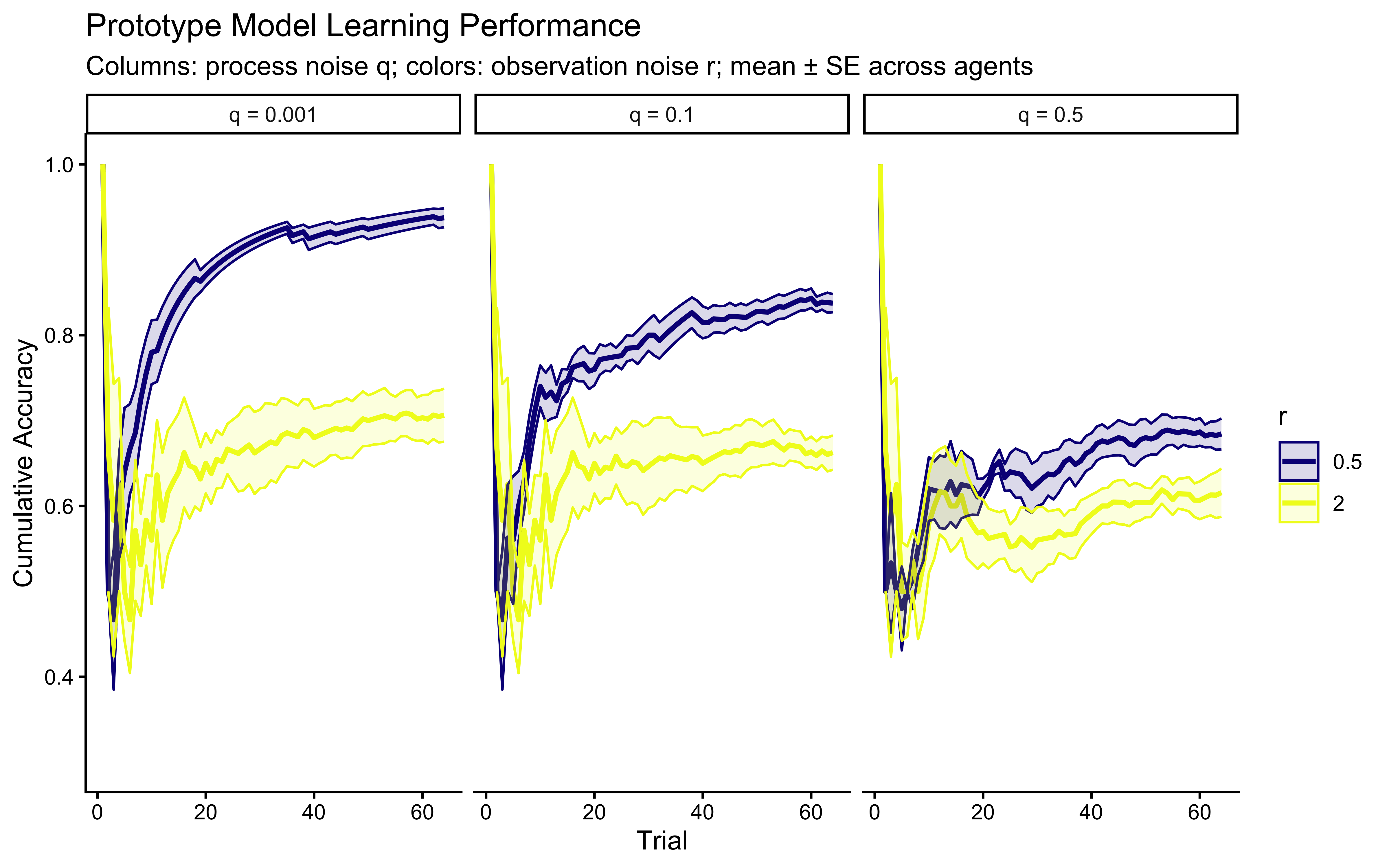
**Interpretation**: The panel structure separates the effects of $r$ (colors) and $q$ (columns). Horizontally (fixed $q$), higher $r$ slows learning and lowers asymptotic accuracy. Vertically (fixed $r$), higher $q$ introduces persistent uncertainty — the model cannot converge to a stable prototype, so accuracy may plateau below ceiling or even oscillate slightly. When $q = 0$ the model reduces to a static-target kalman filter (assumptions of categories as static). The key pedagogical point: $q$ and $r$ are not redundant — they affect different phases of the learning curve and, in non-stationary environments, should become separately identifiable. But we should have learned a lesson from the previous chapter and not assume: let's see if they are identifiable in practice.
### Visualizing Prototype Evolution
Where do the prototypes end up? Let's track their movement and uncertainty over trials.
```{r ch13_track_prototypes}
# Track prototype means and covariance matrices over the course of learning.
# Returns a tibble with one row per (trial × category).
track_prototypes <- function(r_value, obs, cat_one,
                             q_value = 0,
                             initial_mu = NULL, initial_sigma_diag = 10.0) {
  n_trials  <- nrow(obs)
  n_features <- ncol(obs)

  if (is.null(initial_mu)) {
    mu0_init <- rep(2.5, n_features)
    mu1_init <- rep(2.5, n_features)
  } else {
    mu0_init <- initial_mu[[1]]
    mu1_init <- initial_mu[[2]]
  }
  prototype_cat_0 <- list(mu = mu0_init, sigma = diag(initial_sigma_diag, n_features))
  prototype_cat_1 <- list(mu = mu1_init, sigma = diag(initial_sigma_diag, n_features))
  r_matrix        <- diag(r_value, n_features)

  history <- list()

  for (i in seq_len(n_trials + 1)) {
    history[[length(history) + 1]] <- tibble(
      trial      = i, category = 0,
      feature1_mean = prototype_cat_0$mu[1],
      feature2_mean = prototype_cat_0$mu[2],
      cov_matrix    = list(prototype_cat_0$sigma)
    )
    history[[length(history) + 1]] <- tibble(
      trial      = i, category = 1,
      feature1_mean = prototype_cat_1$mu[1],
      feature2_mean = prototype_cat_1$mu[2],
      cov_matrix    = list(prototype_cat_1$sigma)
    )

    if (i <= n_trials) {
      # Prediction step
      prototype_cat_0$sigma <- prototype_cat_0$sigma + diag(q_value, n_features)
      prototype_cat_1$sigma <- prototype_cat_1$sigma + diag(q_value, n_features)

      current_obs <- as.numeric(obs[i, ])
      true_cat    <- cat_one[i]
      if (true_cat == 1) {
        upd <- multivariate_kalman_update(prototype_cat_1$mu, prototype_cat_1$sigma,
                                          current_obs, r_matrix)
        prototype_cat_1$mu    <- upd$mu
        prototype_cat_1$sigma <- upd$sigma
      } else {
        upd <- multivariate_kalman_update(prototype_cat_0$mu, prototype_cat_0$sigma,
                                          current_obs, r_matrix)
        prototype_cat_0$mu    <- upd$mu
        prototype_cat_0$sigma <- upd$sigma
      }
    }
  }
  bind_rows(history)
}

# Ellipse helper for uncertainty visualization
get_ellipse <- function(mu, sigma, level = 0.68) {
  mu    <- as.numeric(mu)
  sigma <- as.matrix(sigma)
  if (length(mu) != 2 || !all(dim(sigma) == c(2, 2))) return(NULL)
  ev <- eigen(sigma, symmetric = TRUE, only.values = TRUE)$values
  if (any(ev <= 1e-6)) sigma <- sigma + diag(ncol(sigma)) * 1e-6
  pts <- tryCatch(
    ellipse::ellipse(sigma, centre = mu, level = level),
    error = function(e) NULL
  )
  if (is.null(pts)) return(NULL)
  as_tibble(pts) |> setNames(c("feature1_mean", "feature2_mean"))
}

# Use a fixed seed-1 schedule for the trajectory visualization
traj_schedule <- make_subject_schedule(stimulus_info, n_blocks, seed = 1)

prototype_trajectory <- track_prototypes(
  r_value            = 1.0,
  q_value            = 0.05,
  obs                = as.matrix(traj_schedule[, c("height", "position")]),
  cat_one            = traj_schedule$category_feedback,
  initial_mu         = list(rep(2.5, 2), rep(2.5, 2)),
  initial_sigma_diag = 10.0
)

final_prototypes    <- prototype_trajectory |> filter(trial == max(trial))

ellipse_data <- final_prototypes |>
  rowwise() |>
  mutate(ell = list(get_ellipse(c(feature1_mean, feature2_mean), cov_matrix[[1]]))) |>
  ungroup() |>
  filter(!map_lgl(ell, is.null)) |>
  unnest(ell)

ggplot() +
  geom_point(data = stimulus_info,
             aes(x = position, y = height, color = factor(category_true),
                 shape = factor(category_true)),
             size = 3, alpha = 0.5) +
  geom_path(
    data = prototype_trajectory |> filter(trial <= total_trials),
    aes(x = feature2_mean, y = feature1_mean,
        group = category, color = factor(category)),
    linetype = "dashed",
    arrow = arrow(type = "closed", length = unit(0.08, "inches"), angle = 20)
  ) +
  geom_point(data = final_prototypes,
             aes(x = feature2_mean, y = feature1_mean, color = factor(category)),
             size = 4, shape = 18) +
  geom_path(data = ellipse_data,
            aes(x = feature2_mean, y = feature1_mean,
                group = category, color = factor(category)),
            alpha = 0.7, linewidth = 0.8) +
  scale_color_manual(values = c("0" = "#0072B2", "1" = "#D55E00"), name = "Category") +
  scale_shape_manual(values = c("0" = 16, "1" = 17), name = "Category") +
  labs(
    title    = "Prototype Learning Trajectory (Kalman Filter, r = 1.0)",
    subtitle = "Prototypes start at (2.5, 2.5). Dashed lines show path; ellipses show final 68% uncertainty.",
    x = "Position Feature", y = "Height Feature"
  ) +
  coord_cartesian(
    xlim = range(c(stimulus_info$position, prototype_trajectory$feature2_mean)) + c(-0.5, 0.5),
    ylim = range(c(stimulus_info$height,   prototype_trajectory$feature1_mean)) + c(-0.5, 0.5)
  )
```
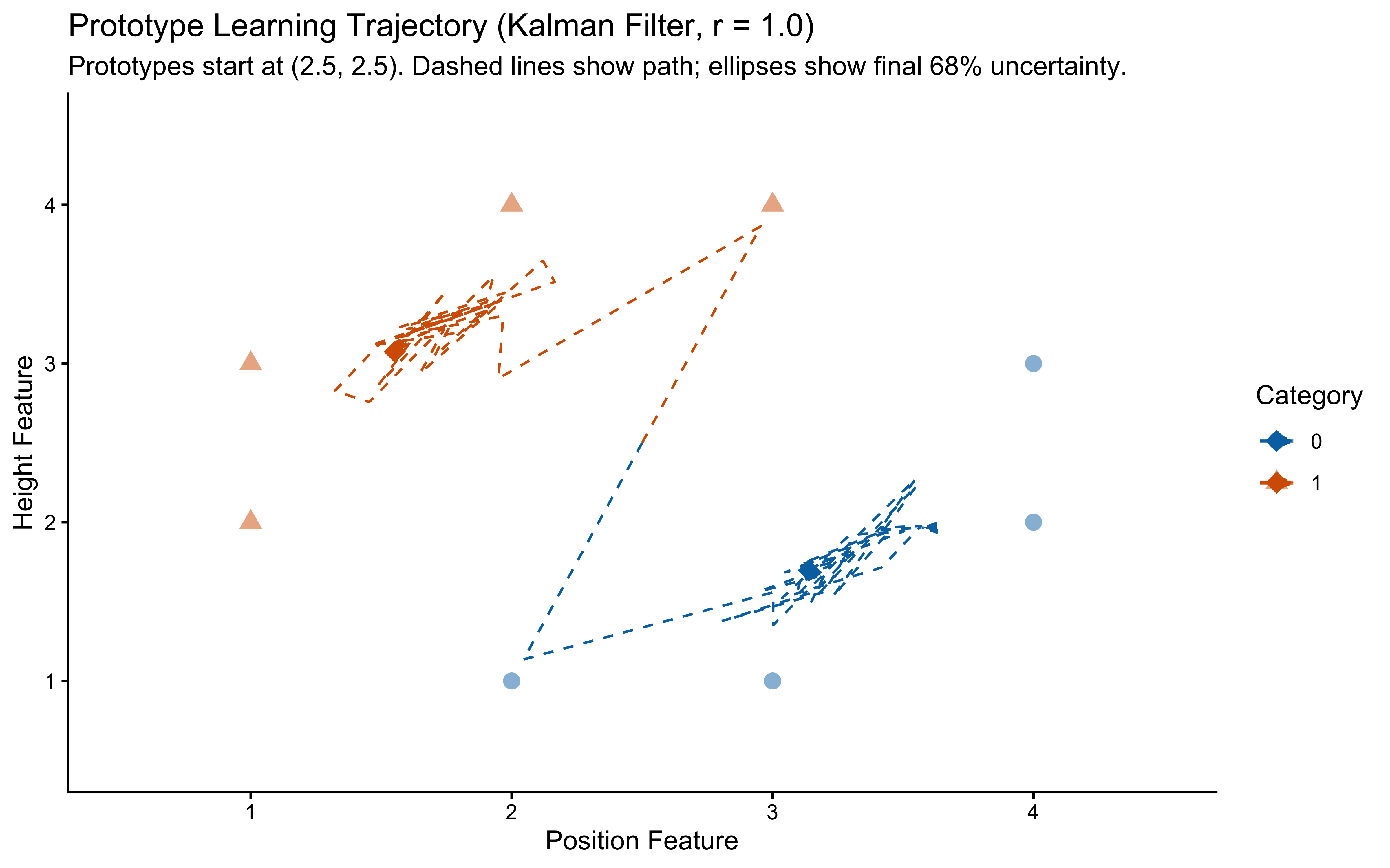
**Interpretation**: The dashed lines show the path the prototypes took during learning (starting from (2.5, 2.5), the center of the feature space). The final prototype locations are marked with diamonds, and the ellipses represent the model's final uncertainty (68% confidence) about the true prototype location for each category. We see the prototypes moving towards the center of their respective category members and uncertainty shrinking over time — exactly the incremental, variance-reducing Bayesian update the Kalman filter implements. The shrinking ellipses indicate that once the agent has seen enough exemplars, the covariances are small enough that further learning is negligible, and the prototypes are effectively frozen.
---
## Prior Predictive Check
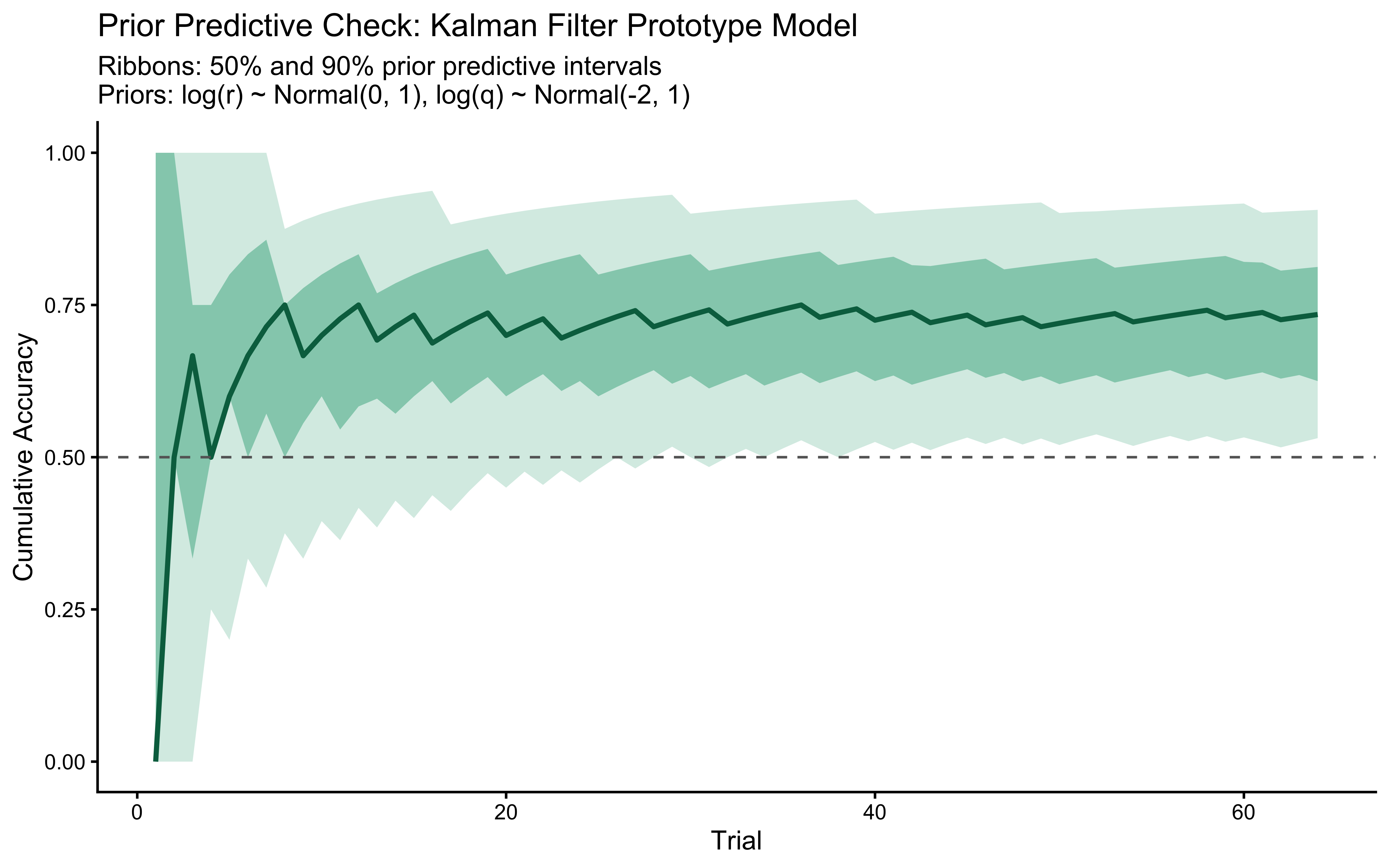
Before fitting any data, we verify that the prior on `log_r` generates only scientifically plausible learning trajectories. We draw $S = 500$ values from $\log r \sim \text{Normal}(0, 1)$ — implying $r \in (0.13, 7.4)$ at $\pm 2$ SD — simulate one agent per draw, and plot the envelope.
```{r ch13_prior_predictive_check}
n_ppc_samples <- 500

ppc_log_r  <- rnorm(n_ppc_samples, LOG_R_PRIOR_MEAN, LOG_R_PRIOR_SD)
ppc_log_q  <- rnorm(n_ppc_samples, LOG_Q_PRIOR_MEAN, LOG_Q_PRIOR_SD)
ppc_r      <- exp(ppc_log_r)
ppc_q      <- exp(ppc_log_q)
ppc_sched  <- make_subject_schedule(stimulus_info, n_blocks, seed = 999)

prior_pred_curves <- map_dfr(seq_len(n_ppc_samples), function(s) {
  res <- prototype_kalman(
    r_value   = ppc_r[s],
    q_value   = ppc_q[s],
    obs       = as.matrix(ppc_sched[, c("height", "position")]),
    cat_one   = ppc_sched$category_feedback,
    initial_mu = list(rep(2.5, 2), rep(2.5, 2))
  )
  tibble(
    sample_id = s,
    trial     = seq_len(nrow(ppc_sched)),
    correct   = as.integer(res$sim_response == ppc_sched$category_feedback)
  ) |>
    mutate(cum_acc = cumsum(correct) / row_number())
})

ppc_summary <- prior_pred_curves |>
  group_by(trial) |>
  summarise(
    q05 = quantile(cum_acc, 0.05), q25 = quantile(cum_acc, 0.25),
    q50 = median(cum_acc),
    q75 = quantile(cum_acc, 0.75), q95 = quantile(cum_acc, 0.95),
    .groups = "drop"
  )

ggplot(ppc_summary, aes(x = trial)) +
  geom_ribbon(aes(ymin = q05, ymax = q95), fill = "#009E73", alpha = 0.20) +
  geom_ribbon(aes(ymin = q25, ymax = q75), fill = "#009E73", alpha = 0.40) +
  geom_line(aes(y = q50), color = "#006D4E", linewidth = 1) +
  geom_hline(yintercept = 0.5, linetype = "dashed", color = "grey40") +
  scale_y_continuous(limits = c(0, 1)) +
  labs(
    title    = "Prior Predictive Check: Kalman Filter Prototype Model",
    subtitle = "Ribbons: 50% and 90% prior predictive intervals\nPriors: log(r) ~ Normal(0, 1), log(q) ~ Normal(-2, 1)",
    x = "Trial", y = "Cumulative Accuracy"
  )
```
The prior predictive envelope spans chance performance (uninformative $r$ draws) through near-ceiling accuracy (informative $r$ draws), without implying impossible behavior such as sustained below-chance performance. Not a hard bar to pass, but a good start.
---
## The Prototype Model in Stan
Simulations help us understand the model, but we want to fit it to experimental data to estimate its parameters. The primary free parameter is the observation noise variance `r_value`. We implement the Kalman filter prototype model in Stan to estimate `r_value` (on the log scale) from data.
### Some implementation notes
### Kalman filter in the transformed parameters
The prototype model has two parameters — `log_r` and `log_q`. Given both and the observed data (stimuli and feedback), the *entire* Kalman filter state is deterministic: prototype means, prototype covariances, and the per-trial choice probability $p_i$ all follow algebraically from `log_r` and the trial sequence. Whenever a quantity depends on a parameter but is otherwise deterministic, it belongs in `transformed parameters` (evaluated once per leapfrog step) rather than `transformed data` (which is for parameter-free preprocessing) or `model{}` (which would force a recomputation in `generated quantities`). We follow that rule here, and `log_lik[i]` in `generated quantities` becomes a one-line lookup of `p[i]`.
> **A note on architectural symmetry with the chapter on exemplars.** The previous chapter GCM's choice probabilities were deterministic given the parameters and the data, and therefore belonged in `transformed parameters`. The same is true for the kalman filter model: `prob_cat1[i]` is a transformed parameter, the model block reduces to a single vectorised `bernoulli_lpmf(y | prob_cat1)`, and `log_lik[i]` is a one-line lookup.
#### Path dependence requires LFO-CV
The same path-dependence concern of the previous chapter applies: trial $t$'s choice probability depends on all previous stimuli through the Kalman state, so standard PSIS-LOO is invalid. Unlike previous drafts, we no longer treat that as a caveat to repeat — the LFO-CV machinery from the previous chapter is generalised to the Kalman case in §"Leave-Future-Out Cross-Validation" below.
> **`reduce_sum` and parallelization**: As with the GCM, the Kalman prototype model cannot use `reduce_sum` because successive Kalman steps are causally chained — trial $t$'s contribution to the likelihood depends on the filter state from trials $1, \ldots, t-1$. The entire filter must be computed sequentially. With two parameters (`log_r`, `log_q`) the posterior geometry is 2D, and Pathfinder initialization is still reliable because both parameters are unconstrained scalars with prior-dominated tails.
### Stan Model
```{r ch13_stan_prototype_model}
prototype_single_stan <- "
// Kalman Filter Prototype Model — Single Subject, with Process Noise
// Key design:
//   log_r and log_q are the two parameters (both unconstrained).
//   r_value = exp(log_r): observation noise variance
//   q_value = exp(log_q): process noise / prototype drift rate
//   Kalman loop structure: Predict (add Q) → Decide → Update.
//   The full filter is in transformed parameters so log_lik in generated
//   quantities reads p[i] directly without re-running the filter.

data {
  int<lower=1> ntrials;
  int<lower=1> nfeatures;
  array[ntrials] int<lower=0, upper=1> cat_one;
  array[ntrials] int<lower=0, upper=1> y;
  array[ntrials, nfeatures] real obs;

  vector[nfeatures] initial_mu_cat0;
  vector[nfeatures] initial_mu_cat1;
  real<lower=0> initial_sigma_diag;

  real prior_logr_mean;
  real<lower=0> prior_logr_sd;
  real prior_logq_mean;
  real<lower=0> prior_logq_sd;
}

parameters {
  real log_r;
  real log_q;
}

transformed parameters {
  real<lower=0> r_value = exp(log_r);
  real<lower=0> q_value = exp(log_q);

  array[ntrials] real<lower=1e-9, upper=1-1e-9> p;

  {
    vector[nfeatures] mu_cat0 = initial_mu_cat0;
    vector[nfeatures] mu_cat1 = initial_mu_cat1;
    matrix[nfeatures, nfeatures] sigma_cat0 =
      diag_matrix(rep_vector(initial_sigma_diag, nfeatures));
    matrix[nfeatures, nfeatures] sigma_cat1 =
      diag_matrix(rep_vector(initial_sigma_diag, nfeatures));
    matrix[nfeatures, nfeatures] r_matrix =
      diag_matrix(rep_vector(r_value, nfeatures));
    matrix[nfeatures, nfeatures] q_matrix =
      diag_matrix(rep_vector(q_value, nfeatures));
    matrix[nfeatures, nfeatures] I_mat =
      diag_matrix(rep_vector(1.0, nfeatures));

    for (i in 1:ntrials) {
      vector[nfeatures] x = to_vector(obs[i]);

      // ── Prediction step: add process noise to both categories ──────────
      sigma_cat0 = sigma_cat0 + q_matrix;
      sigma_cat1 = sigma_cat1 + q_matrix;

      // ── Decision ────────────────────────────────────────────────────────
      matrix[nfeatures, nfeatures] cov0 = sigma_cat0 + r_matrix;
      matrix[nfeatures, nfeatures] cov1 = sigma_cat1 + r_matrix;

      real log_p0 = multi_normal_lpdf(x | mu_cat0, cov0);
      real log_p1 = multi_normal_lpdf(x | mu_cat1, cov1);
      real prob1  = exp(log_p1 - log_sum_exp(log_p0, log_p1));

      p[i] = fmax(1e-9, fmin(1 - 1e-9, prob1));

      // ── Update (measurement update for the correct category only) ────────
      if (cat_one[i] == 1) {
        vector[nfeatures] innov = x - mu_cat1;
        matrix[nfeatures, nfeatures] S  = sigma_cat1 + r_matrix;
        matrix[nfeatures, nfeatures] K  = mdivide_right_spd(sigma_cat1, S);
        matrix[nfeatures, nfeatures] IK = I_mat - K;
        mu_cat1    = mu_cat1 + K * innov;
        sigma_cat1 = IK * sigma_cat1 * IK' + K * r_matrix * K';
        sigma_cat1 = 0.5 * (sigma_cat1 + sigma_cat1');
      } else {
        vector[nfeatures] innov = x - mu_cat0;
        matrix[nfeatures, nfeatures] S  = sigma_cat0 + r_matrix;
        matrix[nfeatures, nfeatures] K  = mdivide_right_spd(sigma_cat0, S);
        matrix[nfeatures, nfeatures] IK = I_mat - K;
        mu_cat0    = mu_cat0 + K * innov;
        sigma_cat0 = IK * sigma_cat0 * IK' + K * r_matrix * K';
        sigma_cat0 = 0.5 * (sigma_cat0 + sigma_cat0');
      }
    }
  }
}

model {
  target += normal_lpdf(log_r | prior_logr_mean, prior_logr_sd);
  target += normal_lpdf(log_q | prior_logq_mean, prior_logq_sd);
  target += bernoulli_lpmf(y | p);
}

generated quantities {
  vector[ntrials] log_lik;
  real lprior;
  for (i in 1:ntrials)
    log_lik[i] = bernoulli_lpmf(y[i] | p[i]);
  lprior = normal_lpdf(log_r | prior_logr_mean, prior_logr_sd) +
           normal_lpdf(log_q | prior_logq_mean, prior_logq_sd);
}
"

stan_file_proto_single <- here("stan", "ch13_prototype_single.stan")

write_stan_file(prototype_single_stan, dir = here("stan"),
                basename = "ch13_prototype_single.stan")
mod_prototype_single <- cmdstan_model(stan_file_proto_single)
```
**Key aspects of the Stan implementation:**
* **Parameters block**: Two scalars `log_r` and `log_q`. Positivity constraints are handled by `exp()` in `transformed parameters`.
* **Prediction step**: `sigma_cat0` and `sigma_cat1` each have `q_matrix` added before the decision. With `q_value = 0` this recovers the static-target filter.
* **Transformed parameters**: Runs the full Kalman filter trial-by-trial, updating the two prototype distributions and recording `p[i]` — the probability of choosing Category 1 on trial $i$ — before each trial's update. The update happens on *all* trials (including the last), consistent with the R simulation.
* **Model block**: Priors on `log_r` and `log_q` plus a vectorised Bernoulli likelihood using the pre-computed `p` vector. One line.
* **Generated quantities**: `log_lik[i]` reads directly from `p[i]` — no re-computation of the Kalman filter required.
---
## Fitting the Model to Simulated Data
We use Pathfinder initialization before HMC sampling. Theoretically, it should make the HMC faster to run. I haven't tested that yet for this model, shamefully, but it doesn't hurt to do it.
```{r ch13_fit_single_agent}
# Select one simulated agent with r_value = 2.0, q_value = 0.1
agent_to_fit <- prototype_responses |>
  filter(r_value_true == 2.0, q_value_true == 0.1, agent_id == 1)

stopifnot(nrow(agent_to_fit) == total_trials)

proto_data_single <- list(
  ntrials            = nrow(agent_to_fit),
  nfeatures          = 2L,
  cat_one            = agent_to_fit$category_feedback,
  y                  = agent_to_fit$sim_response,
  obs                = as.matrix(agent_to_fit[, c("height", "position")]),
  initial_mu_cat0    = c(2.5, 2.5),
  initial_mu_cat1    = c(2.5, 2.5),
  initial_sigma_diag = 10.0,
  prior_logr_mean    = LOG_R_PRIOR_MEAN,
  prior_logr_sd      = LOG_R_PRIOR_SD,
  prior_logq_mean    = LOG_Q_PRIOR_MEAN,
  prior_logq_sd      = LOG_Q_PRIOR_SD
)

fit_filepath_single <- here("simmodels", "ch13_proto_single_fit.rds")
if (regenerate_simulations || !file.exists(fit_filepath_single)) {
  pf_single <- mod_prototype_single$pathfinder(
    data = proto_data_single, seed = 123, num_paths = 4, refresh = 0
  )

  fit_proto_single <- mod_prototype_single$sample(
    data            = proto_data_single,
    init            = pf_single,
    seed            = 123,
    chains          = 4,
    parallel_chains = min(4, availableCores()),
    iter_warmup     = 1000,
    iter_sampling   = 1500,
    refresh         = 300,
    adapt_delta     = 0.9
  )
  fit_proto_single$save_object(fit_filepath_single)
  cat("Single-agent prototype fit computed and saved.\n")
} else {
  fit_proto_single <- readRDS(fit_filepath_single)
  cat("Loaded existing single-agent prototype fit.\n")
}
if (!is.null(fit_proto_single)) {
  param_summary <- fit_proto_single$summary(variables = c("log_r", "r_value", "log_q", "q_value"))
  print(param_summary)

  true_r     <- agent_to_fit$r_value_true[1]
  true_log_r <- log(true_r)
  true_q     <- agent_to_fit$q_value_true[1]
  true_log_q <- log(true_q)
  cat("\nTrue log_r =", round(true_log_r, 3), "  True r =", true_r, "\n")
  cat("True log_q =", round(true_log_q, 3), "  True q =", true_q, "\n")
}
```
### MCMC Diagnostic Battery
Before reading anything off the posterior, we need to check our diagnostic table.
```{r ch13_diagnostic_battery_single}
if (!is.null(fit_proto_single)) {
  diag_tbl <- diagnostic_summary_table(
    fit_proto_single,
    params = c("log_r", "r_value", "log_q", "q_value")
  )
  print(diag_tbl)
}
```
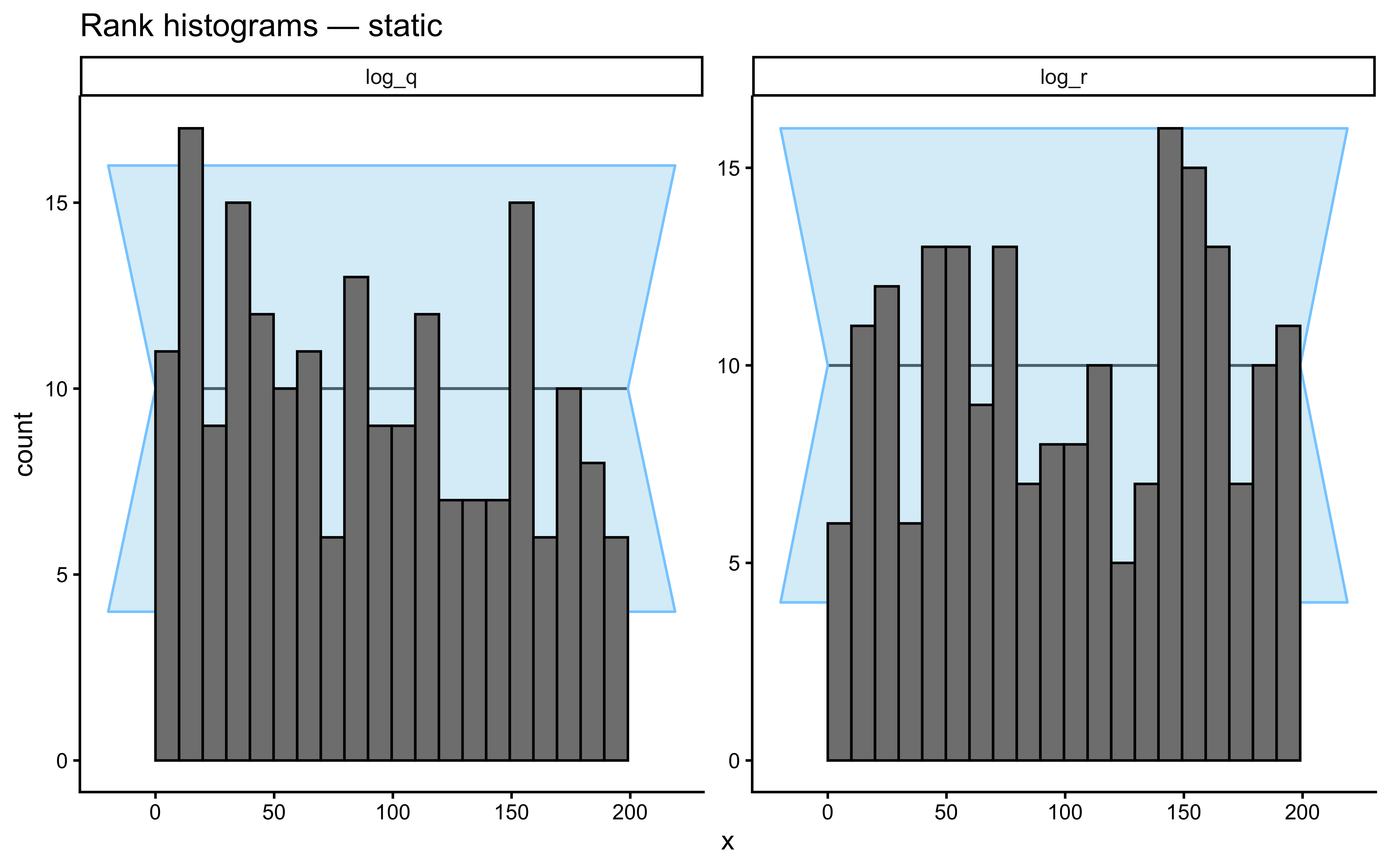
The trace plot grid plus rank histograms remain the primary MCMC diagnostics; we save the joint geometry of `log_r` and `log_q` for after the prior–posterior overlay, where it directly informs the interpretation.
```{r ch13_trace_and_rank}
if (!is.null(fit_proto_single)) {
  p_trace <- bayesplot::mcmc_trace(
    fit_proto_single$draws(c("log_r", "log_q")),
    facet_args = list(ncol = 2)
  ) +
    ggtitle("Trace plots — should look like hairy caterpillars")

  p_rank <- bayesplot::mcmc_rank_overlay(
    fit_proto_single$draws(c("log_r", "log_q")),
    facet_args = list(ncol = 2)
  ) +
    ggtitle("Rank histograms — should be uniform across chains")

  print(p_trace / p_rank)
}
```
### Posterior Predictive Check
The posterior predictive check asks: does the fitted model, when run forward with parameters drawn from the posterior, produce data that look like the observed data? Since `p` is already in `transformed parameters`, we can read posterior draws of the choice probability directly and use them to generate posterior predictive responses.
```{r ch13_ppc}
if (!is.null(fit_proto_single)) {
# Posterior draws of p[i] (one row per draw, one column per trial)
p_draws <- fit_proto_single$draws("p", format = "matrix")
n_draws <- nrow(p_draws)
n_obs <- ncol(p_draws)
# Generate posterior predictive responses
yrep <- matrix(rbinom(n_draws * n_obs, 1, as.vector(p_draws)),
nrow = n_draws, ncol = n_obs)
# Cumulative-accuracy ribbons vs. observed
obs_cum_acc <- cumsum(agent_to_fit$sim_response == agent_to_fit$category_feedback) /
seq_len(n_obs)
# Use "==" directly and add 0 to coerce to numeric without losing matrix dims
yrep_correct <- sweep(yrep, 2, as.numeric(agent_to_fit$category_feedback), "==") + 0
yrep_cum_acc <- t(apply(yrep_correct, 1, function(r) cumsum(r) / seq_along(r)))
cum_acc_summary <- tibble(
trial = seq_len(n_obs),
q05 = apply(yrep_cum_acc, 2, quantile, 0.05),
q25 = apply(yrep_cum_acc, 2, quantile, 0.25),
q50 = apply(yrep_cum_acc, 2, quantile, 0.50),
q75 = apply(yrep_cum_acc, 2, quantile, 0.75),
q95 = apply(yrep_cum_acc, 2, quantile, 0.95),
obs = obs_cum_acc
)
ggplot(cum_acc_summary, aes(x = trial)) +
geom_ribbon(aes(ymin = q05, ymax = q95), fill = "#56B4E9", alpha = 0.20) +
geom_ribbon(aes(ymin = q25, ymax = q75), fill = "#56B4E9", alpha = 0.40) +
geom_line(aes(y = q50), color = "#0072B2", linewidth = 1) +
geom_line(aes(y = obs), color = "#D55E00", linewidth = 1) +
geom_hline(yintercept = 0.5, linetype = "dashed", color = "grey50") +
labs(
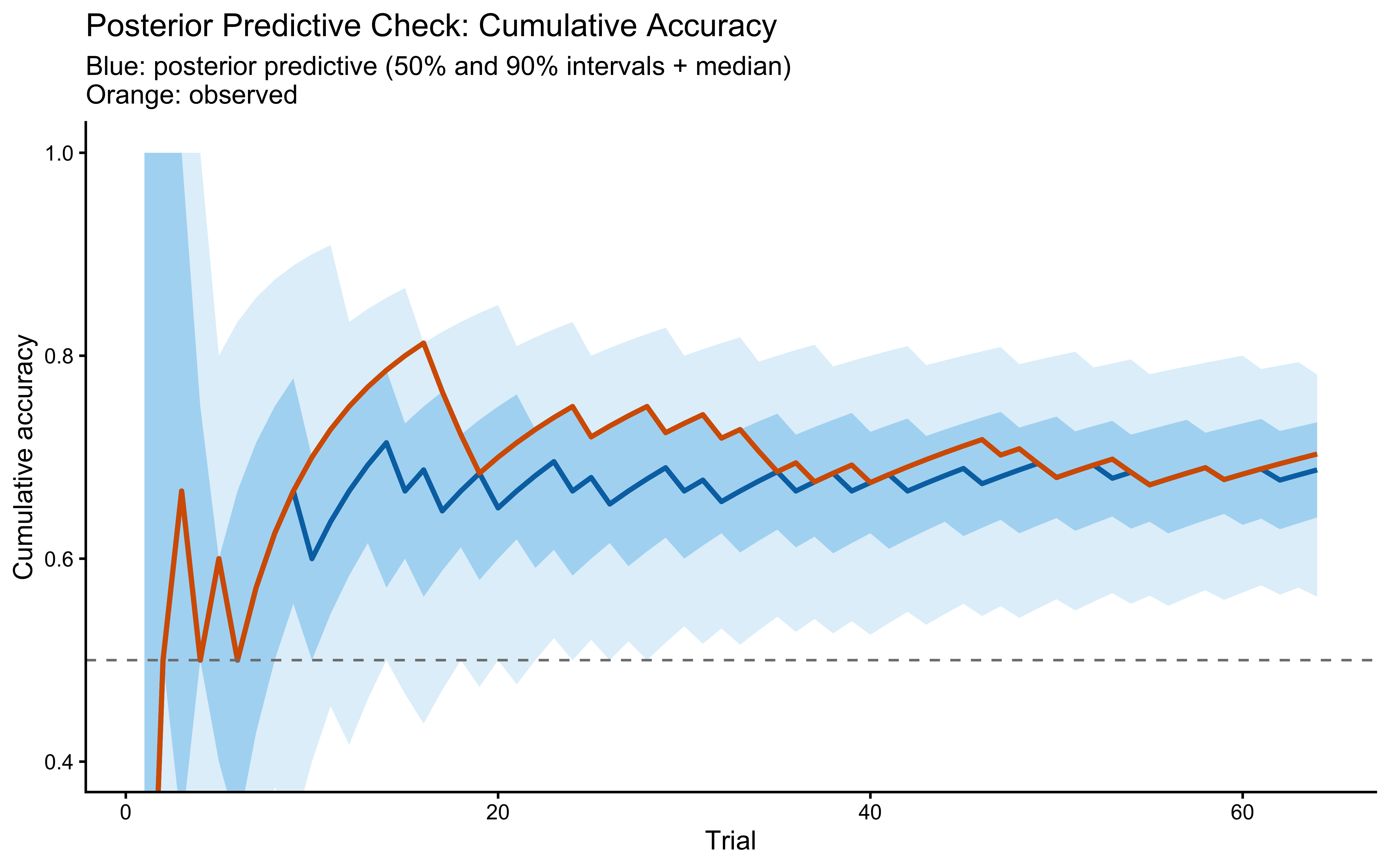
title = "Posterior Predictive Check: Cumulative Accuracy",
subtitle = "Blue: posterior predictive (50% and 90% intervals + median)\nOrange: observed",
x = "Trial", y = "Cumulative accuracy"
) +
coord_cartesian(ylim = c(0.4, 1))
}
```
The observed cumulative-accuracy curve should sit comfortably inside the posterior predictive band. If it drifts to the edge, the model is missing structure that the data carry — the most likely candidate being a separate decisional-noise term that the single $r$ parameter cannot capture.
### Prior–Posterior Update Plot
Did the data teach the model anything? We overlay prior and posterior densities on both the *computational scale* (`log_r`, `log_q`, where the priors were defined) and the *interpretable scale* (`r`, `q`, where the cognitive interpretation lives). Heavy overlap means the data were uninformative; a narrow posterior far from the truth means the model is confidently wrong.
```{r ch13_prior_posterior_update}
if (!is.null(fit_proto_single)) {
draws_df <- as_draws_df(
fit_proto_single$draws(c("log_r", "r_value", "log_q", "q_value"))
)
set.seed(7)
n_prior <- nrow(draws_df)
prior_logr <- rnorm(n_prior, LOG_R_PRIOR_MEAN, LOG_R_PRIOR_SD)
prior_r <- exp(prior_logr)
prior_logq <- rnorm(n_prior, LOG_Q_PRIOR_MEAN, LOG_Q_PRIOR_SD)
prior_q <- exp(prior_logq)
prior_post_df <- bind_rows(
tibble(scale = "log_r", value = prior_logr, source = "prior"),
tibble(scale = "log_r", value = draws_df$log_r, source = "posterior"),
tibble(scale = "r", value = prior_r, source = "prior"),
tibble(scale = "r", value = draws_df$r_value, source = "posterior"),
tibble(scale = "log_q", value = prior_logq, source = "prior"),
tibble(scale = "log_q", value = draws_df$log_q, source = "posterior"),
tibble(scale = "q", value = prior_q, source = "prior"),
tibble(scale = "q", value = draws_df$q_value, source = "posterior")
) |>
mutate(scale = factor(scale, levels = c("log_r", "r", "log_q", "q")))
true_lines <- tibble(
scale = factor(c("log_r", "r", "log_q", "q"),
levels = c("log_r", "r", "log_q", "q")),
value = c(true_log_r, true_r, true_log_q, true_q)
)
ggplot(prior_post_df, aes(x = value, fill = source, color = source)) +
geom_density(alpha = 0.4, linewidth = 0.6) +
geom_vline(data = true_lines,
aes(xintercept = value),
color = "red", linetype = "dashed") +
facet_wrap(~ scale, scales = "free", ncol = 2) +
scale_fill_manual(values = c(prior = "#999999", posterior = "#009E73")) +
scale_color_manual(values = c(prior = "#666666", posterior = "#006D4E")) +
labs(
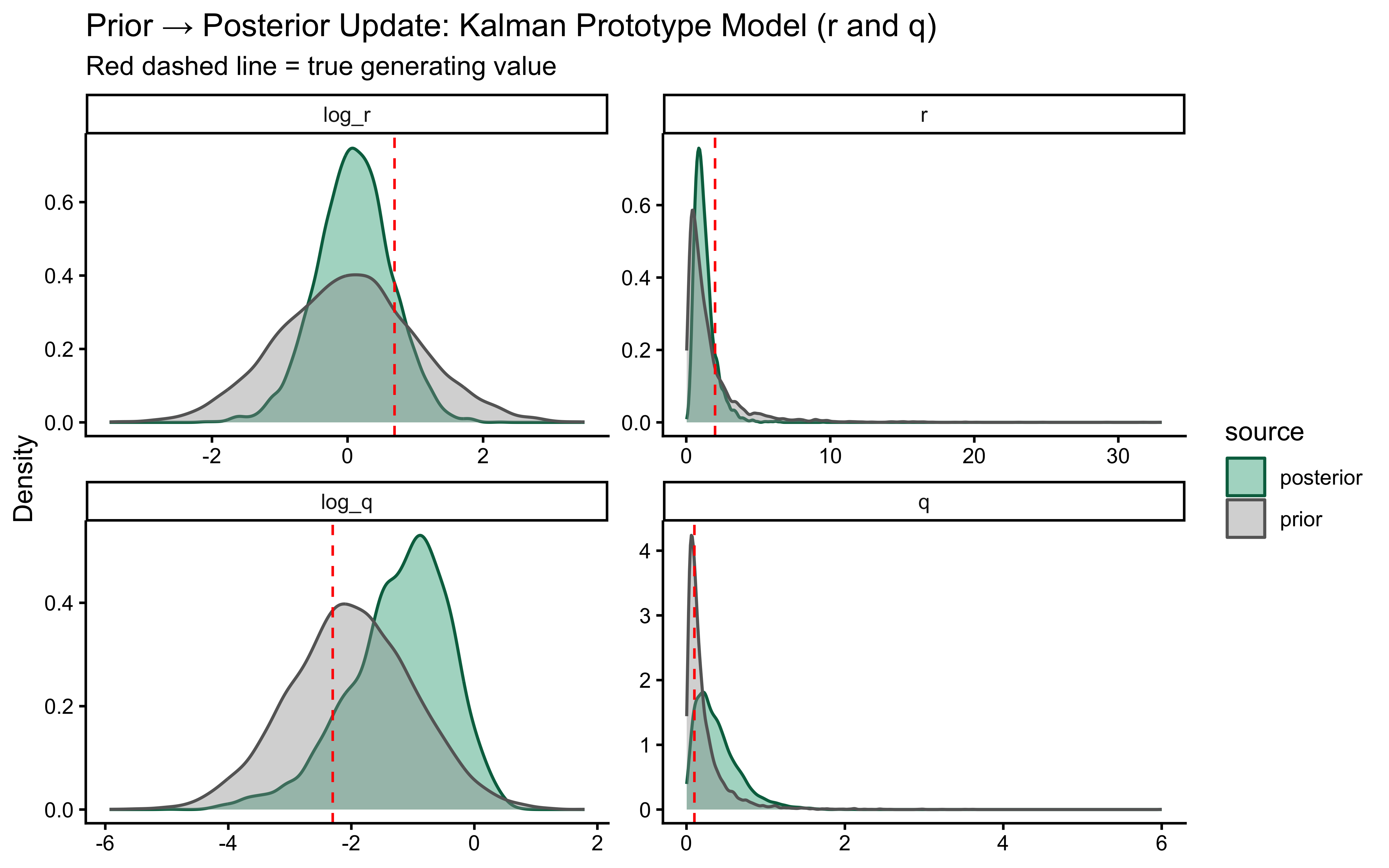
title = "Prior → Posterior Update: Kalman Prototype Model (r and q)",
subtitle = "Red dashed line = true generating value",
x = NULL, y = "Density"
)
}
```
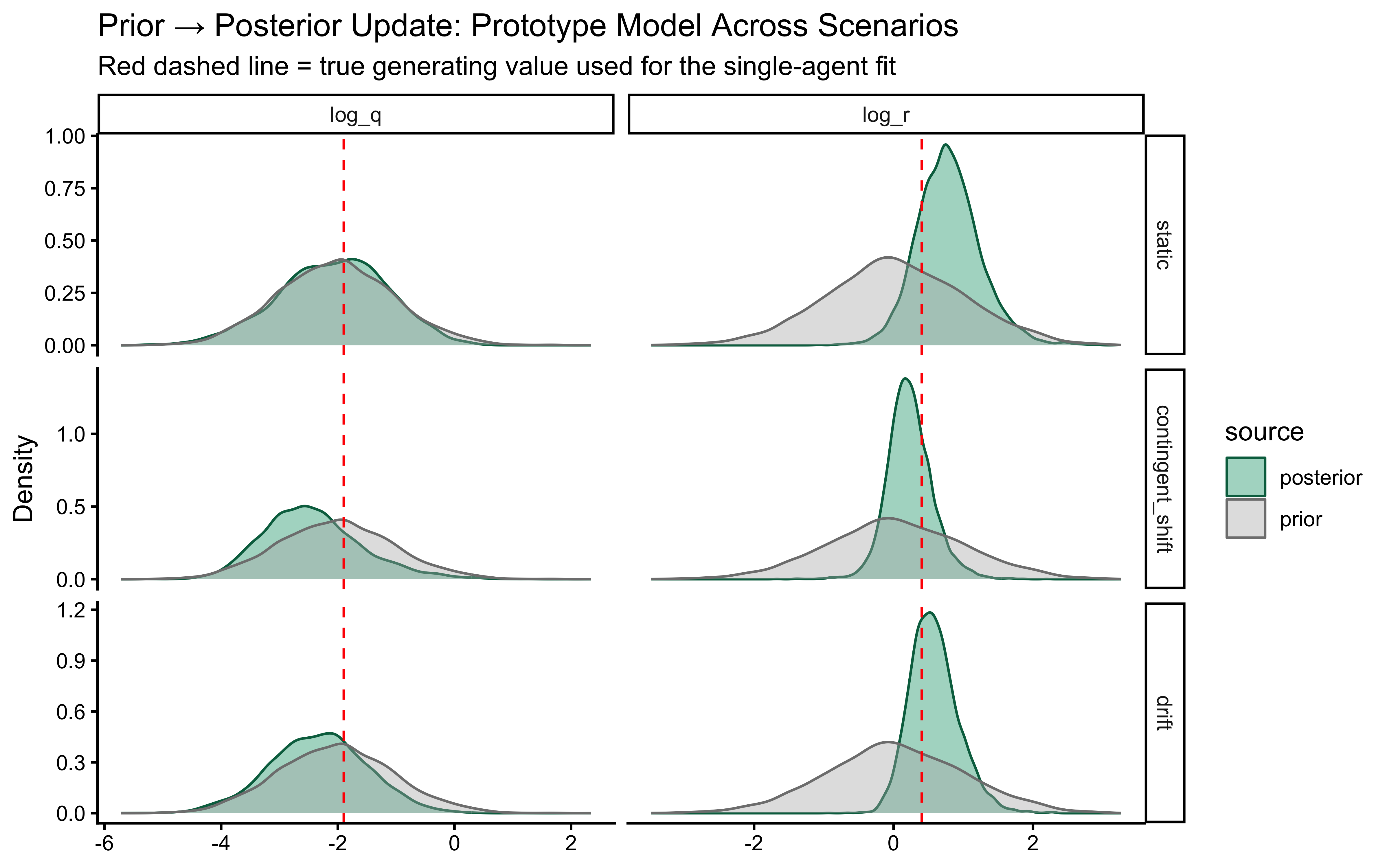
The two parameters update very differently. On `log_r`, the posterior is clearly tighter than the prior and the true value sits well inside the posterior mass — modest but real information gain, with no sign of confident error. On the `r` scale the prior is so heavy-tailed that the contraction is visually compressed into the bulk near zero; the posterior is mostly a sharper version of the prior's left mode, which is the right behaviour given a single subject's worth of trials.
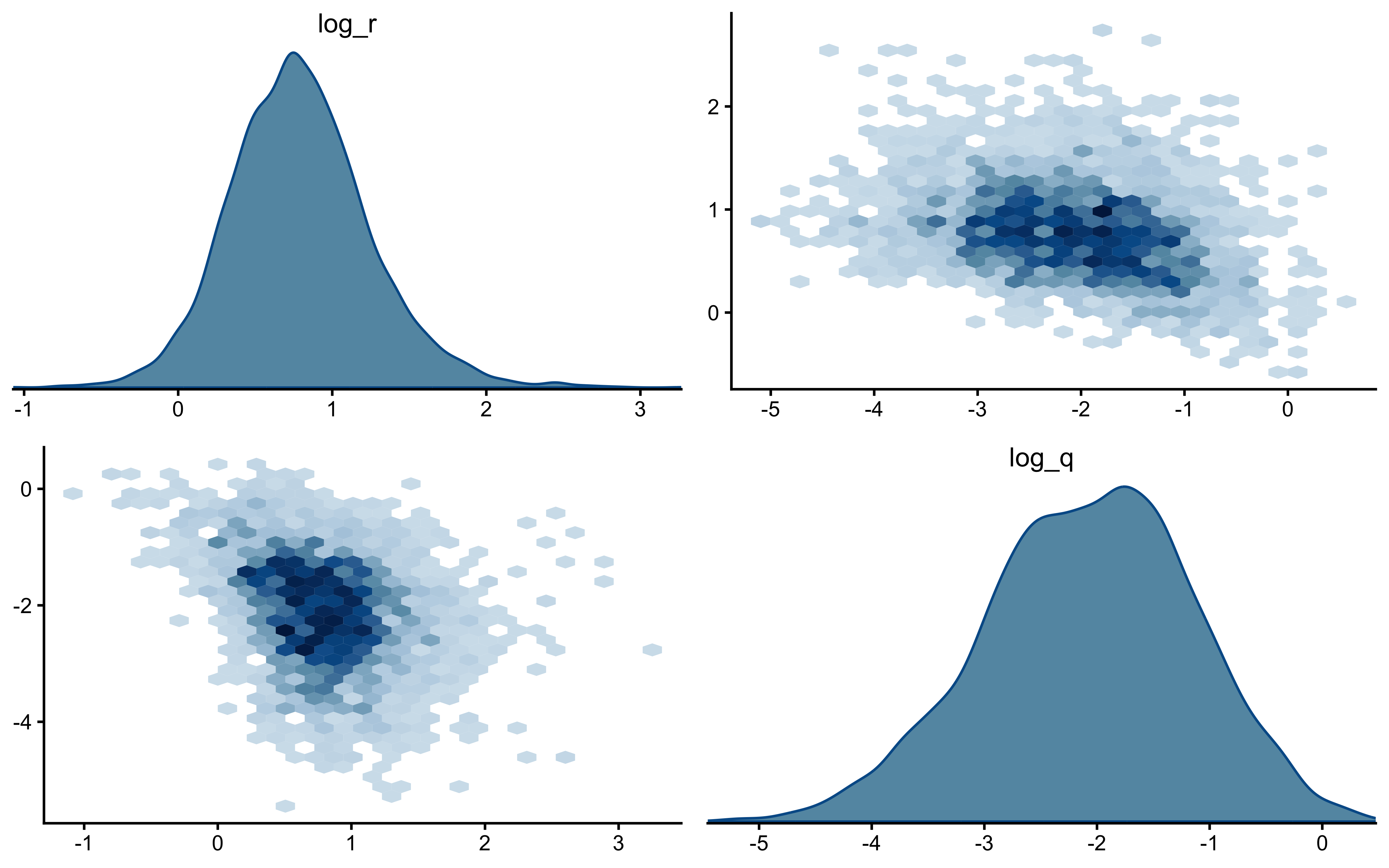
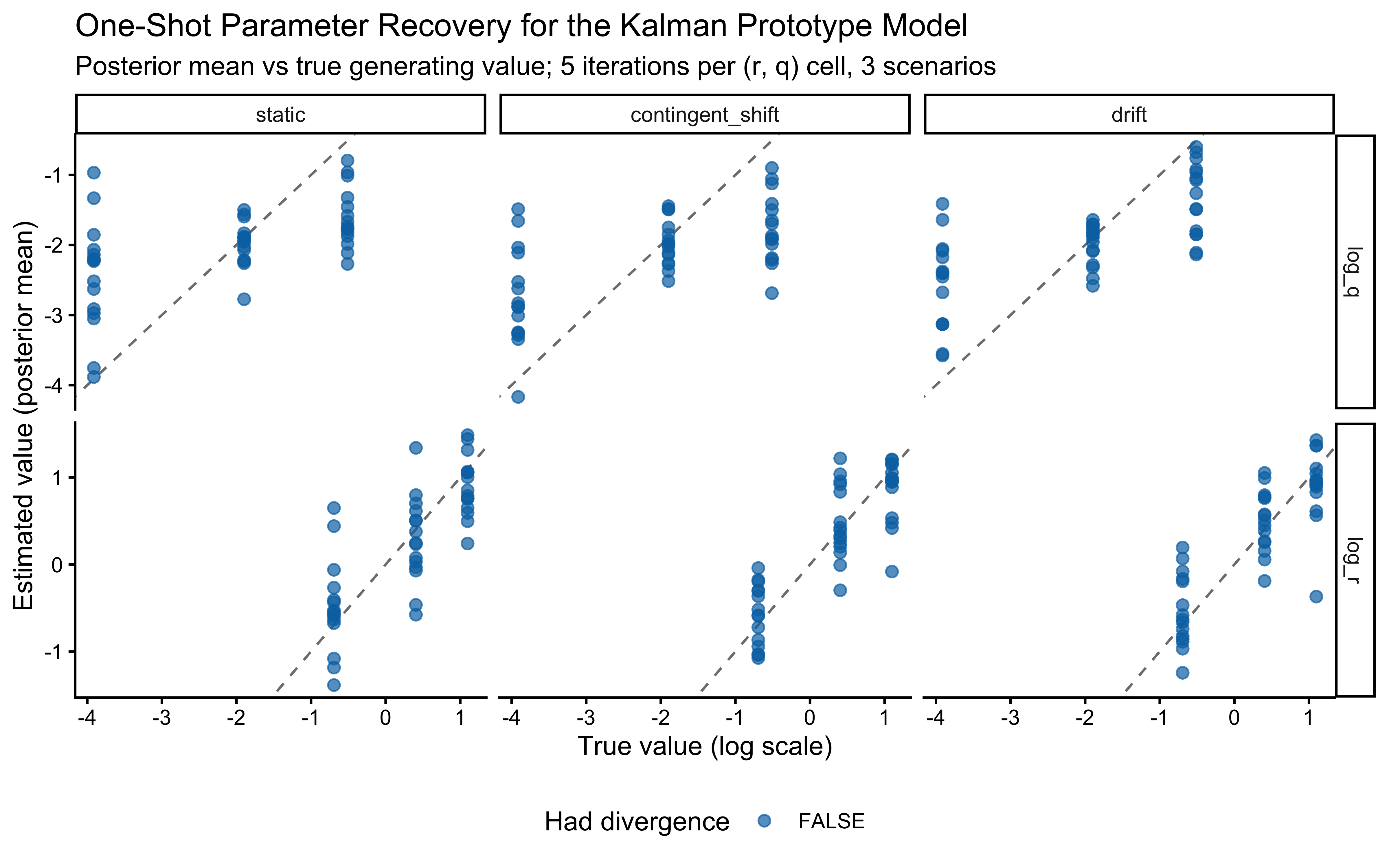
`log_q` is the more interesting panel. The posterior has shifted noticeably *to the right* of the prior, with its mode near $-1$ while the true value sits around $-2.3$ in the posterior's left tail. The data were informative — the posterior is not just the prior — but they pulled $q$ toward larger values than truly generated the sequence. This is the kind of mild, prior-dominated bias one expects when a single trajectory under-determines the process-noise scale: many $(r, q)$ combinations explain the choices about equally well, and the posterior settles in the high-likelihood ridge rather than at the truth. The pairs plot below is the direct way to assess that likely ridge; SBC across many simulated agents is what will tell us whether the offset is systematic.
```{r ch13_pairs}
if (!is.null(fit_proto_single)) {
  bayesplot::mcmc_pairs(
    fit_proto_single$draws(c("log_r", "log_q")),
    diag_fun     = "dens",
    off_diag_fun = "scatter",
    np           = nuts_params(fit_proto_single)
  )
}
```
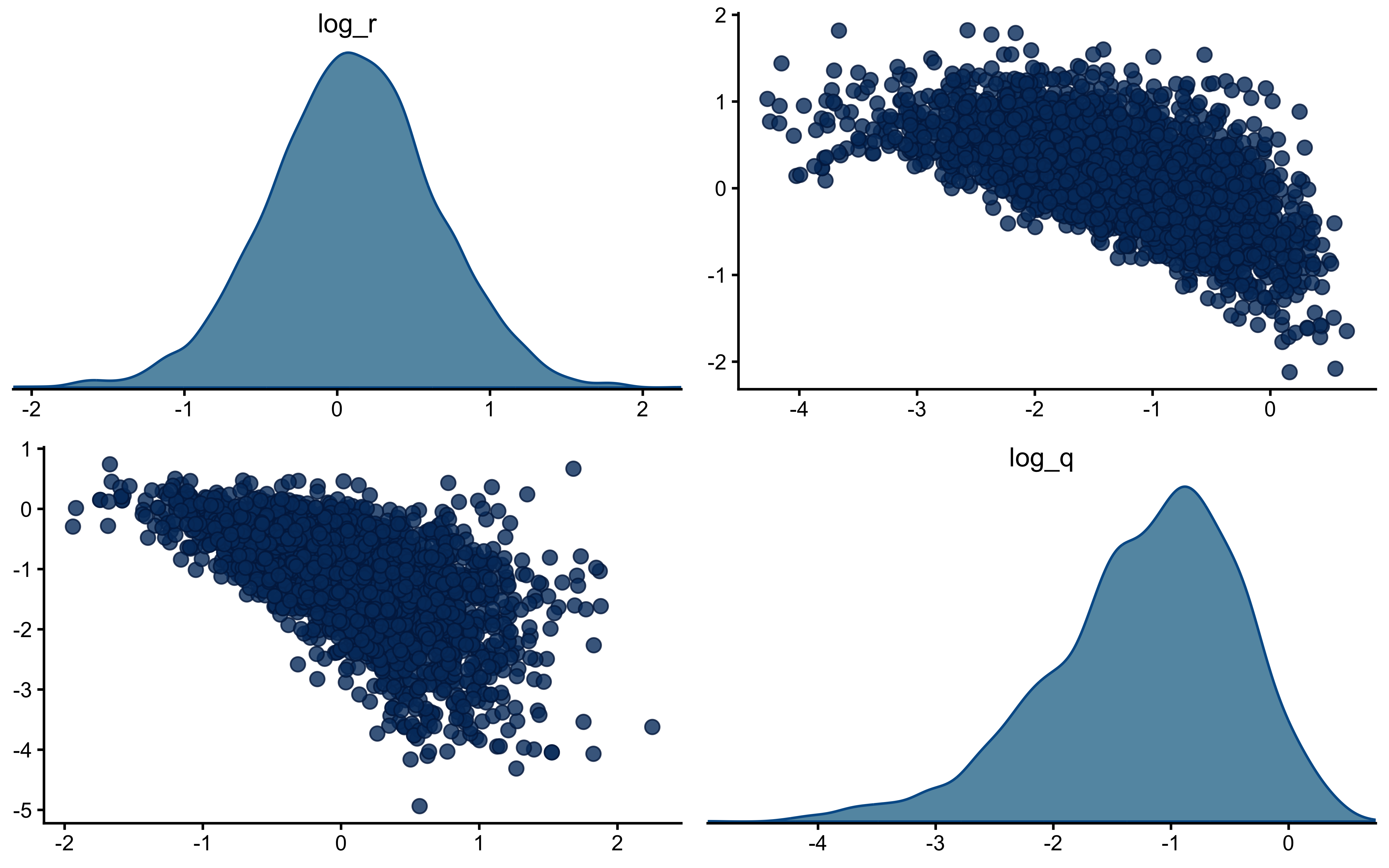
The off-diagonal scatter shows the ridge plainly: `log_r` and `log_q` are clearly negatively correlated, with a fan that opens toward small `log_q` (low process noise paired with high observation noise). Along that ridge, decreasing $q$ and increasing $r$ leave the predicted choice probabilities largely unchanged — a smaller process step combined with noisier readout produces the same trial-by-trial behaviour as a larger process step with cleaner readout. That is exactly why the marginal posterior on `log_q` can sit above the true value while still fitting the choices well: the truth lies somewhere on this ridge, and a single subject's data are not enough to pin down where. What should we do? We could try hierarchical pooling across subjects, or - likely to work - change the experimental setup more dynamic categories, and more trials could help.
### Randomised LOO-PIT Calibration
For continuous outcomes the preferred calibration check is LOO-PIT. For binary outcomes the equivalent is the *randomised* LOO-PIT (Säilynoja et al. 2022), which avoids the degenerate two-bin distribution that plain LOO-PIT produces on Bernoulli data. Chapter 13 implements this for the GCM; we apply the same construction here.
```{r ch13_loo_pit_randomized}
if (!is.null(fit_proto_single)) {
# PSIS-LOO weights from log_lik
log_lik_mat <- fit_proto_single$draws("log_lik", format = "matrix")
# FIX: Add save_psis = TRUE so the weight matrix is retained
loo_obj <- loo::loo(log_lik_mat, cores = 4, save_psis = TRUE)
log_w <- loo::weights.importance_sampling(loo_obj$psis_object,
normalize = TRUE,
log = TRUE)
# Posterior draws of choice probability
p_draws <- fit_proto_single$draws("p", format = "matrix")
# Per-observation LOO predictive probability of cat 1
loo_p_cat1 <- vapply(seq_len(ncol(p_draws)), function(i) {
sum(exp(log_w[, i]) * p_draws[, i])
}, numeric(1))
y_obs <- agent_to_fit$sim_response
# Randomised PIT for binary y:
# if y == 1: U ~ Uniform(1 - p, 1)
# if y == 0: U ~ Uniform(0, 1 - p)
set.seed(2026)
rloo_pit <- vapply(seq_along(y_obs), function(i) {
p_i <- loo_p_cat1[i]
if (y_obs[i] == 1) runif(1, 1 - p_i, 1) else runif(1, 0, 1 - p_i)
}, numeric(1))
p_pit <- ggplot(tibble(rloo_pit = rloo_pit), aes(x = rloo_pit)) +
geom_histogram(aes(y = after_stat(density)), bins = 20,
fill = "#56B4E9", color = "white") +
geom_hline(yintercept = 1, linetype = "dashed", color = "red") +
labs(
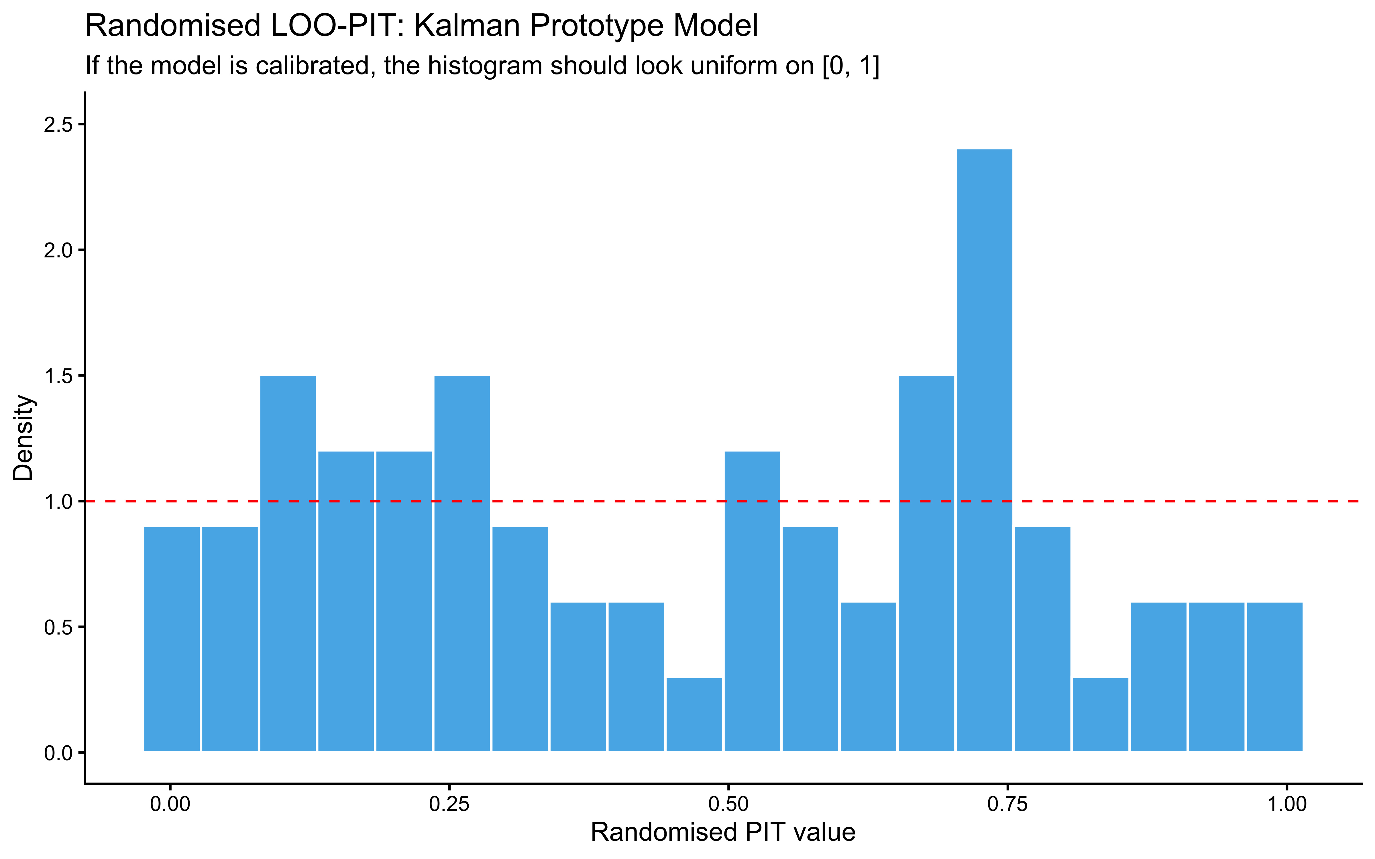
title = "Randomised LOO-PIT: Kalman Prototype Model",
subtitle = "If the model is calibrated, the histogram should look uniform on [0, 1]",
x = "Randomised PIT value", y = "Density"
) +
coord_cartesian(ylim = c(0, 2.5))
print(p_pit)
}
```
A roughly uniform histogram is the calibration target. The histogram here is bumpy but not pathological: bars hover around the uniform reference (red dashed line at density 1), with no systematic U-shape (which would flag overconfidence), no central hump (underconfidence), and no monotone skew (a directional bias the model has not captured). The two visible spikes — one near $0.1$–$0.25$ and a taller one near $0.7$ — are the kind of small-sample noise expected from 64 binary trials; with only a few dozen randomised PIT values, individual bins fluctuate considerably even under perfect calibration. The mild excess on the lower-middle and upper-middle and the slight under-density in the tails ($>0.85$) are worth keeping in mind, but with this much data they do not constitute evidence of miscalibration. The check kinda passes; the meaningful calibration question is whether this pattern persists across many simulated agents, which is what SBC will answer.
### LOO with Pareto-k as a Diagnostic, Not a Predictive Score
```{r ch13_loo_single}
if (!is.null(fit_proto_single)) {
  loo_proto <- loo::loo(log_lik_mat, cores = 4)
  print(loo_proto)
  plot(loo_proto, label_points = TRUE,
       main = "PSIS-LOO Pareto-k: Kalman Prototype Model")
}
```
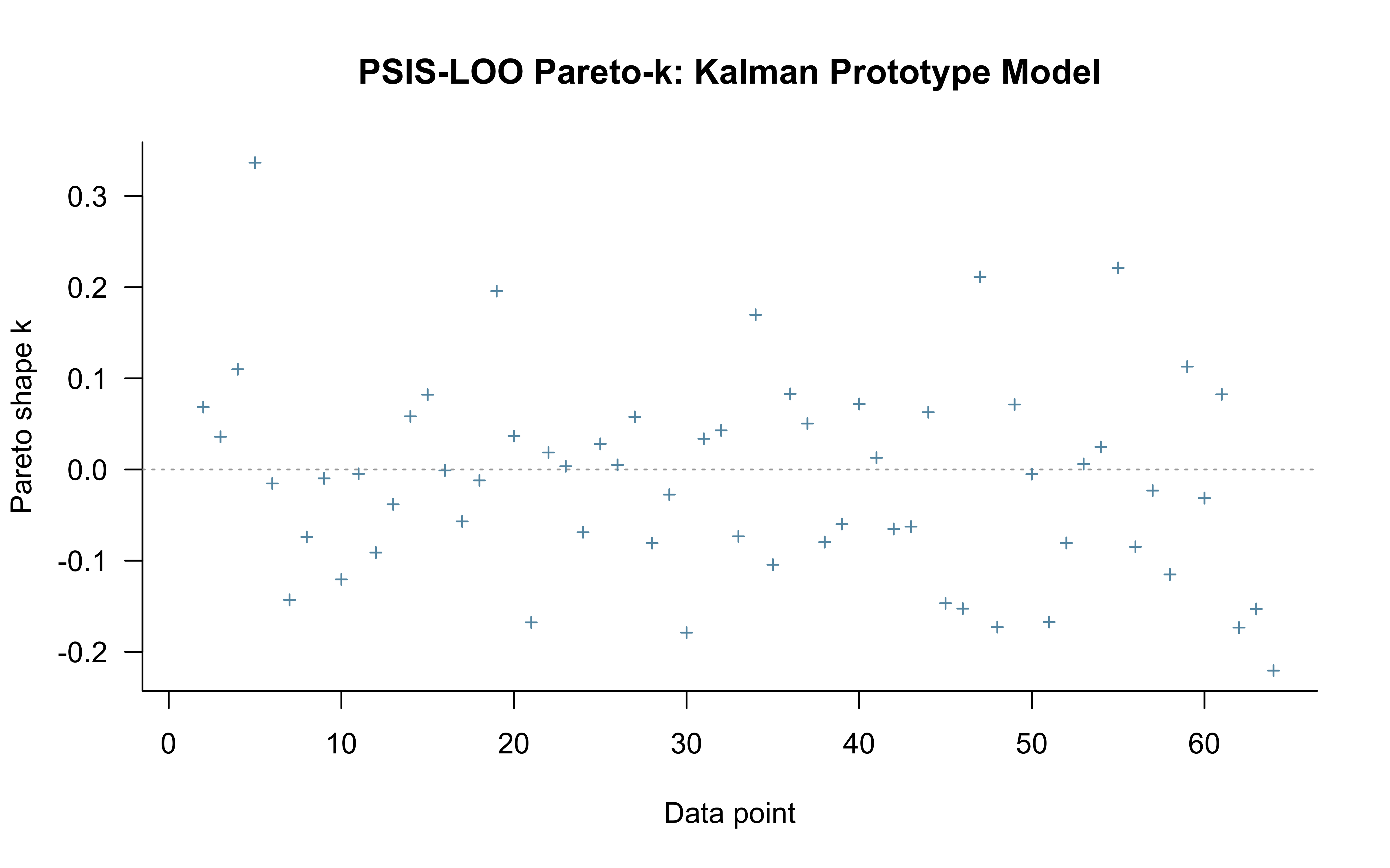
> **⚠️ Reframing PSIS-LOO for sequential models.** The Kalman filter is path-dependent: trial $t$'s choice probability depends on the entire filter state from trials $1, \ldots, t-1$. Standard PSIS-LOO is *not* a valid measure of out-of-sample predictive accuracy here — leaving out trial $t$ implicitly conditions on a counterfactual filter state that the model never actually saw. We compute it anyway, for two reasons: (1) the **Pareto-$\hat{k}$ values are still informative as a localisation diagnostic** — high $\hat{k}$ at specific trials flags observations the model cannot easily reconstruct from the rest, which can reveal where the structural assumptions are stressed; (2) compatibility with downstream tooling. The actual predictive evaluation is done by LFO-CV in the next subsection. The numeric ELPD reported by `loo()` should not be taken as a generalisation estimate.
**What we see here.** The Pareto-$\hat{k}$ scatter is essentially flat: 63 of 64 points sit between roughly $-0.2$ and $+0.35$, with $p_\text{loo} = 1.1$ (close to the parameter count, as expected for a well-behaved fit) and a minimum ESS of $\sim$5000 across observations. Read as a localisation diagnostic, this is the good case — no individual trial is a structural outlier that the rest of the data cannot reconstruct. The single "very bad" entry counted in the diagnostic table (1.6%) is the first trial, which has no preceding history and so is not a meaningful PSIS-LOO target; the plot above clips it. The headline $\text{elpd}_\text{loo} = -38.8$ is reported for completeness but, per the reframing above, should not be interpreted as out-of-sample predictive accuracy — that is what LFO-CV in the next subsection actually measures.
### Leave-Future-Out Cross-Validation: Inheriting and Generalising the GCM Implementation
For sequential models, LOO is invalid and LFO-CV is the correct alternative (Bürkner, Gabry, & Vehtari 2020). Chapter 13 implements PSIS-LFO for the GCM as `psis_lfo_gcm()`. The Kalman prototype model has the same path-dependence structure but a much cheaper per-trial cost, so LFO-CV is even more tractable here. Below is the same algorithm specialised to the prototype model and saved as `psis_lfo_kalman()`. The two functions share an interface so later chapters with empirical analyses can call either through a common front-end.
The algorithm (Bürkner et al. 2020 Algorithm 1):
1. Choose a minimum training window $L$ (we use $L = 16$, two blocks of the Kruschke task).
2. Fit the model once on $y_{1:L}$. This is the *reference fit*.
3. For each $t = L+1, \ldots, T$:
a. Use the reference fit's posterior draws $\theta^{(s)}$ to compute the importance ratio for re-weighting $\theta$ from $p(\theta \mid y_{1:t-1})$ relative to the reference.
b. Smooth the ratios with PSIS, check Pareto $\hat{k}$.
c. If $\hat{k} \leq 0.7$, accept the ratios and use them to evaluate $\log p(y_t \mid y_{1:t-1})$.
d. If $\hat{k} > 0.7$, **refit** the model on $y_{1:t-1}$, update the reference, and continue.
4. Return pointwise ELPD, the refit history, and the $\hat{k}$ trajectory.
```{r ch13_psis_lfo_kalman}
# psis_lfo_kalman(): Leave-future-out CV for the Kalman prototype model.
# Mirrors psis_lfo_gcm() from Chapter 12. Returns pointwise ELPD across the
# evaluation window, the indices at which a refit was triggered, and the
# Pareto-k trajectory.
psis_lfo_kalman <- function(stan_data,
                            stan_model,
                            L           = 16,    # min training window
                            k_thresh    = 0.7,   # PSIS-k refit threshold
                            iter_warmup = 800,
                            iter_sample = 1000,
                            chains      = 2,
                            seed        = 1) {
  T_total <- stan_data$ntrials

  # Helper: build a stan_data list restricted to trials 1:t
  truncate_data <- function(d, t) {
    out <- d
    out$ntrials <- t
    out$cat_one <- d$cat_one[1:t]
    out$y       <- d$y[1:t]
    out$obs     <- d$obs[1:t, , drop = FALSE]
    out
  }

  # Helper: fit on y_{1:t}
  refit <- function(t) {
    d_t <- truncate_data(stan_data, t)
    pf  <- tryCatch(
      stan_model$pathfinder(data = d_t, num_paths = 4, refresh = 0,
                            seed = seed + t),
      error = function(e) NULL
    )
    init_val <- if (!is.null(pf)) pf else 0.5
    stan_model$sample(
      data            = d_t,
      init            = init_val,
      seed            = seed + t,
      chains          = chains,
      parallel_chains = chains,
      iter_warmup     = iter_warmup,
      iter_sampling   = iter_sample,
      refresh         = 0,
      adapt_delta     = 0.9
    )
  }

  # Helper: given a fitted model, evaluate log_lik at trial t
  # using cmdstanr's $generate_quantities() so we don't re-MCMC.
  # Helper: given a fitted model, evaluate log_lik at trial t
  eval_log_lik_at <- function(fit_ref, t) {
    # Build the "extended" data that includes trial t in the likelihood
    d_ext <- truncate_data(stan_data, t)

    # FIX: Call generate_quantities on stan_model, not fit_ref
    gq <- stan_model$generate_quantities(
      fitted_params = fit_ref,
      data          = d_ext,
      seed          = seed + t,
      parallel_chains = chains
    )

    # log_lik[t] for each posterior draw
    ll_mat <- gq$draws("log_lik", format = "matrix")
    ll_mat[, t]
  }

  # ── Initial fit on the minimum window ─────────────────────────────────────
  cat("Initial LFO fit on trials 1 to", L, "...\n")
  fit_ref <- refit(L)
  ref_window <- L

  # Storage
  pointwise_elpd <- rep(NA_real_, T_total)
  k_hat_traj     <- rep(NA_real_, T_total)
  refit_at       <- integer(0)

  # ── Sequential evaluation ─────────────────────────────────────────────────
  log_ratios_accum <- numeric(0)  # log p(y_{ref+1:t-1} | theta) accumulation
  for (t in (L + 1):T_total) {
    # Build importance ratios for theta_ref vs theta_{1:t-1}
    if (length(log_ratios_accum) == 0) {
      log_w <- rep(0, posterior::ndraws(fit_ref$draws()))
    } else {
      log_w <- log_ratios_accum  # raw log ratios; psis() handles normalization
    }

    # PSIS smoothing
    psis_obj <- tryCatch(
      loo::psis(log_ratios = matrix(log_w, ncol = 1), r_eff = 1),
      error = function(e) NULL
    )
    k_hat <- if (!is.null(psis_obj)) loo::pareto_k_values(psis_obj) else Inf
    k_hat_traj[t] <- k_hat

    if (!is.finite(k_hat) || k_hat > k_thresh) {
      # Refit on y_{1:t-1}
      cat("  trial", t, ": k_hat =", round(k_hat, 2), "→ refitting\n")
      fit_ref <- refit(t - 1)
      ref_window <- t - 1
      refit_at <- c(refit_at, t)
      log_ratios_accum <- numeric(0)
      log_w <- rep(0, posterior::ndraws(fit_ref$draws()))
      psis_obj <- loo::psis(log_ratios = matrix(log_w, ncol = 1), r_eff = 1)
    }

    # Evaluate log p(y_t | y_{1:t-1}, theta) for each draw
    ll_t <- eval_log_lik_at(fit_ref, t)

    # Importance-weighted estimate of log p(y_t | y_{1:t-1})
    log_w_norm <- as.vector(weights(psis_obj, normalize = TRUE, log = TRUE))
    pointwise_elpd[t] <- matrixStats::logSumExp(log_w_norm + ll_t)

    # Accumulate log p(y_t | theta) for the next iteration's importance ratio
    if (length(log_ratios_accum) == 0) {
      log_ratios_accum <- ll_t
    } else {
      log_ratios_accum <- log_ratios_accum + ll_t
    }
  }

  list(
    pointwise_elpd = pointwise_elpd,
    refit_at       = refit_at,
    k_hat_traj     = k_hat_traj,
    L              = L,
    elpd_lfo       = sum(pointwise_elpd, na.rm = TRUE),
    n_refits       = length(refit_at)
  )
}
```
> **Note on the importance-ratio accumulation.** The trick that makes PSIS-LFO efficient is that the importance ratio for $p(\theta \mid y_{1:t-1})$ vs the reference $p(\theta \mid y_{1:L})$ is a *running product*: for each new trial $t$ we just multiply the existing per-draw weight by $p(y_{t-1} \mid \theta)$. We never need to refit so long as the smoothed Pareto-$\hat{k}$ stays below the threshold. When it crosses 0.7, we refit and reset the running product. The accumulation in `log_ratios_accum` above implements this — every time we evaluate `log_lik[t]`, we add it to the cumulative log-ratio for the next iteration.
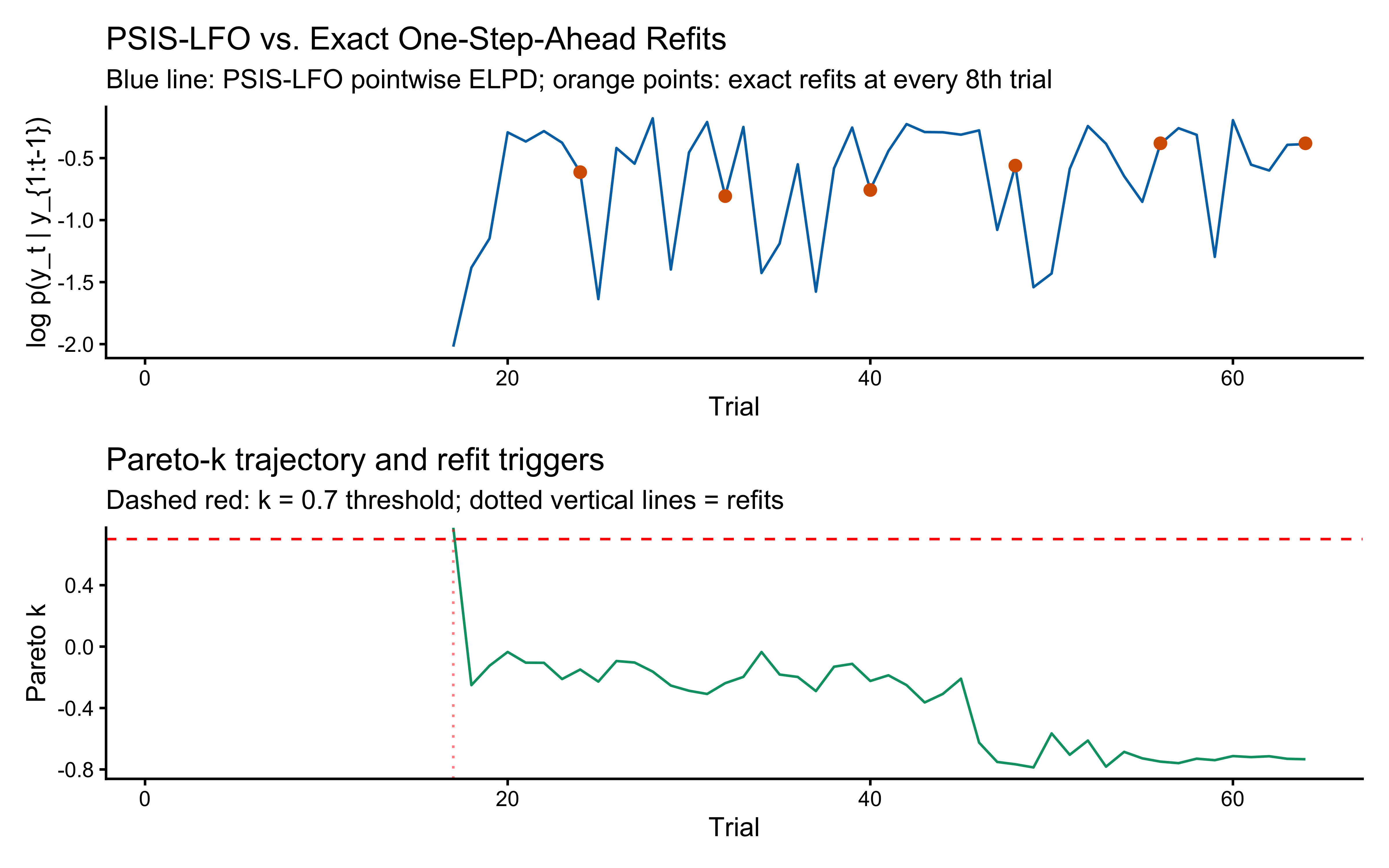
We now run this on the same single-agent fit, and validate it against *exact* one-step-ahead refits at every 8th trial. If PSIS-LFO is doing its job, the two ELPD curves should agree closely.
```{r ch13_lfo_run}
lfo_cache_file <- here("simdata", "ch13_lfo_kalman_results.rds")
if (regenerate_simulations || !file.exists(lfo_cache_file)) {
  cat("Running PSIS-LFO for the prototype model...\n")
  lfo_psis <- psis_lfo_kalman(
    stan_data  = proto_data_single,
    stan_model = mod_prototype_single,
    L          = 16,
    k_thresh   = 0.7
  )

  # ── Exact one-step-ahead refits at every 8th trial ────────────────────────
  exact_t <- seq(24, total_trials, by = 8)
  exact_elpd <- numeric(length(exact_t))
  for (k in seq_along(exact_t)) {
    t <- exact_t[k]
    cat("  exact refit at t =", t, "\n")
    d_t <- proto_data_single
    d_t$ntrials <- t - 1
    d_t$cat_one <- proto_data_single$cat_one[1:(t - 1)]
    d_t$y       <- proto_data_single$y[1:(t - 1)]
    d_t$obs     <- proto_data_single$obs[1:(t - 1), , drop = FALSE]

    pf  <- tryCatch(
      mod_prototype_single$pathfinder(data = d_t, num_paths = 4, refresh = 0),
      error = function(e) NULL
    )
    init_val <- if (!is.null(pf)) pf else 0.5
    fit_t <- mod_prototype_single$sample(
      data = d_t, init = init_val, chains = 2, parallel_chains = 2,
      iter_warmup = 800, iter_sampling = 1000, refresh = 0, adapt_delta = 0.9
    )

    # Evaluate log_lik at trial t
    d_ext <- proto_data_single
    d_ext$ntrials <- t
    d_ext$cat_one <- proto_data_single$cat_one[1:t]
    d_ext$y       <- proto_data_single$y[1:t]
    d_ext$obs     <- proto_data_single$obs[1:t, , drop = FALSE]

    # ── THE FIX: Called on mod_prototype_single instead of fit_t ──
    gq <- mod_prototype_single$generate_quantities(fitted_params = fit_t, data = d_ext)

    ll_mat <- gq$draws("log_lik", format = "matrix")
    exact_elpd[k] <- matrixStats::logSumExp(ll_mat[, t]) - log(nrow(ll_mat))
  }

  saveRDS(list(lfo_psis = lfo_psis,
               exact_t = exact_t, exact_elpd = exact_elpd),
          lfo_cache_file)
  cat("LFO results computed and saved.\n")
} else {
  cached <- readRDS(lfo_cache_file)
  lfo_psis <- cached$lfo_psis
  exact_t <- cached$exact_t
  exact_elpd <- cached$exact_elpd
  cat("Loaded existing LFO results.\n")
}
if (exists("lfo_psis")) {
  cat("PSIS-LFO sum ELPD:", round(lfo_psis$elpd_lfo, 2), "\n")
  cat("Number of refits triggered:", lfo_psis$n_refits,
      "out of", total_trials - lfo_psis$L, "trials\n")

  # Plot: PSIS-LFO pointwise vs exact refits
  comp_df <- tibble(
    trial    = seq_along(lfo_psis$pointwise_elpd),
    psis_elpd = lfo_psis$pointwise_elpd
  )
  exact_df <- tibble(trial = exact_t, exact_elpd = exact_elpd)

  p_lfo <- ggplot(comp_df, aes(x = trial, y = psis_elpd)) +
    geom_line(color = "#0072B2") +
    geom_point(data = exact_df,
               aes(x = trial, y = exact_elpd),
               color = "#D55E00", size = 2) +
    labs(
      title    = "PSIS-LFO vs. Exact One-Step-Ahead Refits",
      subtitle = "Blue line: PSIS-LFO pointwise ELPD; orange points: exact refits at every 8th trial",
      x = "Trial", y = "log p(y_t | y_{1:t-1})"
    )

  # Plot: Pareto-k trajectory and refit triggers
  k_df <- tibble(trial = seq_along(lfo_psis$k_hat_traj),
                 k_hat = lfo_psis$k_hat_traj)
  refit_df <- tibble(trial = lfo_psis$refit_at)

  p_k <- ggplot(k_df, aes(x = trial, y = k_hat)) +
    geom_line(color = "#009E73") +
    geom_hline(yintercept = 0.7, linetype = "dashed", color = "red") +
    geom_vline(data = refit_df, aes(xintercept = trial),
               linetype = "dotted", color = "red", alpha = 0.5) +
    labs(
      title    = "Pareto-k trajectory and refit triggers",
      subtitle = "Dashed red: k = 0.7 threshold; dotted vertical lines = refits",
      x = "Trial", y = "Pareto k"
    )

  print(p_lfo / p_k)
}
```
**Reading the output.** The blue line is the PSIS-LFO pointwise ELPD over the evaluation window ($t = L+1, \ldots, T$ with $L = 16$); the orange points are exact one-step-ahead refits at every 8th trial. The two sit on top of each other within Monte Carlo noise: the orange points fall on the blue trace at every trial they appear, so the importance-sampling shortcut is reproducing the exact one-step-ahead predictive density rather than drifting away from it.
The Pareto-$\hat{k}$ panel tells the same story more directly. There is one initial spike at $t = L+1 = 17$ that crosses the $0.7$ threshold and triggers the first (and only) refit — the dotted vertical line — which makes sense: extending the reference fit by one trial after only $L$ trials of training data is the regime where importance ratios are most volatile. After that single refit, $\hat{k}$ collapses to negative values and stays well below the threshold for the rest of the sequence, drifting further down (toward $-0.8$) as more data accumulates and the posterior becomes increasingly stable. No further refits are needed, so for this fit PSIS-LFO is essentially free after the first step.
The pointwise ELPD itself shows the expected post-warmup pattern: very negative around $t \approx 17$ (the model has only just begun learning), rapidly rising to a band roughly between $-1.5$ and $-0.3$ as the prototype filter converges, with trial-to-trial variation reflecting harder vs. easier stimuli rather than systematic drift. Summing across the window gives the LFO ELPD that should be used for model comparison in Chapter 15 — *not* the `elpd_loo` from the previous subsection. If, on a different fit or scenario, the two curves diverged systematically or $\hat{k}$ stayed above $0.7$ for many consecutive trials, the exact refit pipeline (slow but unambiguous) is the fallback.
### Prior Sensitivity Analysis
```{r ch13_prior_sensitivity}
if (!is.null(fit_proto_single)) {
  ps <- priorsense::powerscale_sensitivity(fit_proto_single)
  print(ps)
  priorsense::powerscale_plot_dens(fit_proto_single, variables = c("log_r", "r_value", "log_q", "q_value"))
}
```
`powerscale_sensitivity()` perturbs the prior and the likelihood analytically (without re-running MCMC) and reports, for each parameter, a sensitivity index — the cumulative Jensen–Shannon distance between the unperturbed posterior and the perturbed one. A value above $\sim 0.05$ is non-trivial; above $0.1$ is a flag. The "diagnosis" column combines the two columns: large likelihood sensitivity with comparable prior sensitivity is reported as *potential prior–data conflict*; large prior sensitivity with small likelihood sensitivity is reported as *strong prior / weak likelihood*.
For this single-agent fit the numbers tell a coherent story. `log_r` (prior $\psi = 0.08$, likelihood $\psi = 0.10$) and `log_q` (prior $0.08$, likelihood $0.14$) both sit just at or above the soft threshold, with the likelihood doing slightly more of the work — the data are informative, but the prior is not negligible. On the natural scale the picture sharpens: `r_value` is dominated by the likelihood (prior $0.07$, likelihood $0.20$), while `q_value` flips the other way (prior $0.21$, likelihood $0.13$) — the prior on $q$ is materially shaping the posterior, exactly as the prior–posterior overlay and the `log_r`–`log_q` ridge already suggested. Almost every per-trial $p[i]$ is flagged as well, but those flags are induced by the parameter-level fragility flowing through the deterministic Kalman recursion, not by independent likelihood issues at each trial.
Practically, this is not a model failure — it is a small-data diagnosis. With one subject and 64 trials the prior on `log_q` cannot be treated as a passive default; the conclusion about process noise depends on it. The two routes out are the standard ones: tighter priors backed by an explicit justification, or hierarchical pooling across subjects so that `log_q` is informed by the population rather than by a single trajectory along the ridge. The density plot overlays posteriors at $\alpha \in \{0.8, 1, 1.25\}$ for both prior- and likelihood-scaling and confirms the table visually: visible (but not dramatic) shifts on `log_q` and `q_value`, near-overlapping curves on `log_r` and `r_value`.
---
## Simulation-Based Calibration Checks (SBC)
Parameter recovery at specific true values is a necessary but not sufficient validation. SBC checks that the full posterior is correctly calibrated across the entire prior distribution — that if the true `log_r` and `log_q` were drawn from their priors, the posterior would on average contain each true value in the appropriate fraction of its probability mass.
The prototype model's two scalar parameters make the resulting ECDF-difference plot particularly legible: the `log_r` curve should show tight calibration (the data are informative), while the `log_q` curve may be wider under the static paradigm (partial confound with `log_r`).
```{r ch13_sbc_prototype}
sbc_proto_filepath <- here("simdata", "ch13_sbc_proto_results.rds")
if (regenerate_simulations || !file.exists(sbc_proto_filepath)) {
  n_sbc_iterations_proto <- 500   # use >= 1000 for publication-quality SBC

  proto_sbc_generator <- SBC_generator_function(
    function() {
      # 1a. Draw true parameters from their priors
      log_r_true <- rnorm(1, LOG_R_PRIOR_MEAN, LOG_R_PRIOR_SD)
      r_true     <- exp(log_r_true)
      log_q_true <- rnorm(1, LOG_Q_PRIOR_MEAN, LOG_Q_PRIOR_SD)
      q_true     <- exp(log_q_true)

      # 1b. Simulate one dataset with its own randomized schedule
      sbc_sched <- make_subject_schedule(stimulus_info, n_blocks,
                                         seed = sample.int(1e8, 1))
      sim       <- prototype_kalman(
        r_value    = r_true,
        q_value    = q_true,
        obs        = as.matrix(sbc_sched[, c("height", "position")]),
        cat_one    = sbc_sched$category_feedback,
        initial_mu = list(rep(2.5, 2), rep(2.5, 2))
      )

      list(
        variables = list(log_r = log_r_true, log_q = log_q_true),
        generated = list(
          ntrials            = nrow(sbc_sched),
          nfeatures          = 2L,
          cat_one            = as.integer(sbc_sched$category_feedback),
          y                  = as.integer(sim$sim_response),
          obs                = as.matrix(sbc_sched[, c("height", "position")]),
          initial_mu_cat0    = c(2.5, 2.5),
          initial_mu_cat1    = c(2.5, 2.5),
          initial_sigma_diag = 10.0,
          prior_logr_mean    = LOG_R_PRIOR_MEAN,
          prior_logr_sd      = LOG_R_PRIOR_SD,
          prior_logq_mean    = LOG_Q_PRIOR_MEAN,
          prior_logq_sd      = LOG_Q_PRIOR_SD
        )
      )
    }
  )

  proto_sbc_backend <- SBC_backend_cmdstan_sample(
    mod_prototype_single,
    iter_warmup   = 1000,
    iter_sampling = 1000,
    chains        = 2,
    adapt_delta   = 0.9,
    refresh       = 0
  )

  proto_datasets <- generate_datasets(
    proto_sbc_generator,
    n_sims = n_sbc_iterations_proto
  )

  sbc_results_proto <- compute_SBC(
    proto_datasets,
    proto_sbc_backend,
    cache_mode     = "results",
    cache_location = here("simdata", "ch13_sbc_proto_cache"),
    keep_fits      = FALSE
  )
  saveRDS(sbc_results_proto, sbc_proto_filepath)
  cat("SBC prototype results computed and saved.\n")
} else {
  sbc_results_proto <- readRDS(sbc_proto_filepath)
  cat("Loaded existing SBC prototype results.\n")
}
plot_ecdf_diff(sbc_results_proto)
plot_rank_hist(sbc_results_proto)
# ── Diagnostic issue investigation ───────────────────────────────────────────
backend_diags  <- sbc_results_proto$backend_diagnostics
default_diags  <- sbc_results_proto$default_diagnostics |>
  dplyr::select(sim_id, max_rhat, min_ess_to_rank)
true_params_wide <- sbc_results_proto$stats |>
  dplyr::select(sim_id, variable, simulated_value) |>
  tidyr::pivot_wider(names_from = variable, values_from = simulated_value)

diag_df <- backend_diags |>
  dplyr::left_join(default_diags,    by = "sim_id") |>
  dplyr::left_join(true_params_wide, by = "sim_id") |>
  dplyr::mutate(has_issue = n_divergent > 0 | n_max_treedepth > 0 | max_rhat > 1.01)

p_diag_r_q <- ggplot(diag_df, aes(x = log_r, y = log_q, color = has_issue)) +
  geom_point(alpha = 0.7, size = 2) +
  scale_color_manual(values = c("FALSE" = "#0072B2", "TRUE" = "#D55E00")) +
  labs(title    = "Diagnostic Issues in Parameter Space",
       subtitle = "Orange points: divergence, max treedepth, or Rhat > 1.01",
       x = "True log(r)", y = "True log(q)") +
  theme(legend.position = "bottom")

print(p_diag_r_q)
# ── Parameter recovery on SBC simulations ────────────────────────────────────
recovery_df <- sbc_results_proto$stats

p_sbc_recovery <- ggplot(recovery_df, aes(x = simulated_value, y = mean)) +
  geom_point(alpha = 0.4, color = "#0072B2") +
  geom_abline(intercept = 0, slope = 1, color = "red", linetype = "dashed") +
  facet_wrap(~variable, scales = "free") +
  labs(
    title    = "Parameter Recovery Across SBC Simulations",
    subtitle = "Posterior mean vs True generated value",
    x = "True Value (simulated_value)",
    y = "Estimated Value (Posterior Mean)"
  ) +
  theme_bw()

print(p_sbc_recovery)
```
---
## Non-Stationary Environments: When Does $q$ Become Identifiable?
The SBC result above hints at a structural tension. Under the static Kruschke paradigm, $\log r$ shows mild systematic overestimation while $\log q$ exhibits a prior-dominated, overdispersed posterior — ranks cluster at the extremes rather than uniformly across the distribution, indicating the posterior is correctly wide rather than incorrectly confident. Crucially, both curves remain within the simultaneous bands, so the model is *calibrated*: the posterior honestly represents its own uncertainty. But the patterns reveal that $\log q$ is weakly identified when nothing drifts — many $(r, q)$ combinations explain static choices about equally well, and the posterior spreads across a wide range of process-noise values. This is not a coding bug or a sampler problem: it is a genuine identifiability limitation caused by a mismatch between the *parameter* (process noise controlling prototype drift) and the *task* (fixed category centres with no drift to detect).
Three generative processes stress this identifiability question differently. We implement all three and run the full validation battery on each.
As established in the canonical scenario framework introduced in the previous chapter, all three categorization chapters use the same three scenarios in the same order (static → contingent shift → drift), reflecting increasing assumption match between the scenario's data-generating process and the model's structural commitments.
1. **Static Kruschke (baseline).** Fixed category labels. The Kalman filter's process-noise prior assumes smooth Gaussian drift; under stationary data, no amount of $q$ improves fit once transient learning is over. We expect $\log q$ to remain weakly identified — this is the failure case we need to diagnose clearly.
2. **Performance-contingent abrupt shifts.** After the agent reaches a streak of $k$ consecutive correct responses, all category labels flip. Post-flip recovery is *fast* for agents whose $q$ lets the covariance re-inflate after surprise, and *slow* for agents whose $q$ is tiny — so $q$ acquires a direct behavioural signature. But the true process has abrupt jumps, which the filter's Gaussian-drift prior does not literally contain; this is a misspecified-but-informative scenario. Note that these shifts are *endogenous* to the agent's own accuracy — a noisier agent triggers fewer flips and accumulates less information about $q$ (see previous chapter for discussion).
3. **Smooth drift.** Category centres in feature space follow an independent random walk; labels are assigned trial-by-trial by proximity to the current drifted centres. This is the **assumption-matched** scenario: the Kalman filter's generative story (prototypes drift as Gaussian random walks) is now literally true of the environment. We expect $\log q$ to be cleanly identified and SBC to pass.
The three scenarios span the spectrum of assumption match — **none → misspecified → exact** — and the SBC signatures should sort in that order.
### Scenario-Aware Simulator
```{r ch13_scenario_simulator}
simulate_prototype_scenario <- function(r_value, q_value, schedule,
                                        scenario = c("static",
                                                     "contingent_shift",
                                                     "drift"),
                                        streak_target      = 8,
                                        drift_traj         = NULL,
                                        initial_mu_cat0    = c(2.5, 2.5),
                                        initial_mu_cat1    = c(2.5, 2.5),
                                        initial_sigma_diag = 10.0) {
  scenario <- match.arg(scenario)
  ntrials  <- nrow(schedule)
  obs_mat  <- as.matrix(schedule[, c("height", "position")])
  base_lab <- schedule$category_feedback
  nfeat    <- 2L

  mu0    <- initial_mu_cat0
  mu1    <- initial_mu_cat1
  sigma0 <- diag(initial_sigma_diag, nfeat)
  sigma1 <- diag(initial_sigma_diag, nfeat)
  R_mat  <- diag(r_value, nfeat)
  Q_mat  <- diag(q_value, nfeat)
  I_mat  <- diag(nfeat)

  label_flip <- FALSE
  streak     <- 0L

  prob_cat1         <- numeric(ntrials)
  sim_response      <- integer(ntrials)
  observed_feedback <- integer(ntrials)
  label_flip_trace  <- logical(ntrials)

  for (i in seq_len(ntrials)) {
    x <- as.numeric(obs_mat[i, ])

    # ── Prediction step ──────────────────────────────────────────────
    sigma0 <- sigma0 + Q_mat
    sigma1 <- sigma1 + Q_mat

    # ── Decision ─────────────────────────────────────────────────────
    cov0 <- sigma0 + R_mat
    cov1 <- sigma1 + R_mat
    lp0  <- tryCatch(mvtnorm::dmvnorm(x, mean = mu0, sigma = cov0, log = TRUE),
                     error = function(e) -Inf)
    lp1  <- tryCatch(mvtnorm::dmvnorm(x, mean = mu1, sigma = cov1, log = TRUE),
                     error = function(e) -Inf)
    m    <- max(lp0, lp1)
    p    <- exp(lp1 - (m + log(exp(lp0 - m) + exp(lp1 - m))))
    p    <- pmax(1e-9, pmin(1 - 1e-9, p))
    prob_cat1[i]    <- p
    sim_response[i] <- rbinom(1, 1, p)

    # ── Observed feedback depends on the scenario ────────────────────
    fb <- switch(scenario,
      static           = base_lab[i],
      contingent_shift = if (label_flip) 1L - base_lab[i] else base_lab[i],
      drift            = {
        d0 <- sum(abs(x - drift_traj$mu0[i, ]))
        d1 <- sum(abs(x - drift_traj$mu1[i, ]))
        as.integer(d1 < d0)
      }
    )
    observed_feedback[i] <- fb
    label_flip_trace[i]  <- label_flip

    # Update the streak/flip state for the contingent scenario
    if (scenario == "contingent_shift") {
      streak <- if (sim_response[i] == fb) streak + 1L else 0L
      if (streak >= streak_target) { label_flip <- !label_flip; streak <- 0L }
    }

    # ── Measurement update for the observed-feedback category ────────
    if (fb == 1) {
      innov  <- x - mu1
      S      <- sigma1 + R_mat
      K      <- sigma1 %*% solve(S)
      mu1    <- as.numeric(mu1 + K %*% innov)
      IK     <- I_mat - K
      sigma1 <- IK %*% sigma1 %*% t(IK) + K %*% R_mat %*% t(K)
      sigma1 <- (sigma1 + t(sigma1)) / 2
    } else {
      innov  <- x - mu0
      S      <- sigma0 + R_mat
      K      <- sigma0 %*% solve(S)
      mu0    <- as.numeric(mu0 + K %*% innov)
      IK     <- I_mat - K
      sigma0 <- IK %*% sigma0 %*% t(IK) + K %*% R_mat %*% t(K)
      sigma0 <- (sigma0 + t(sigma0)) / 2
    }
  }

  schedule |>
    mutate(
      prob_cat1         = prob_cat1,
      sim_response      = sim_response,
      observed_feedback = observed_feedback,
      label_flip        = label_flip_trace,
      correct           = as.integer(sim_response == observed_feedback)
    )
}
```
### Drift Trajectory Generator
The drift scenario pre-computes a trajectory for both category centres as independent bivariate Gaussian random walks.
```{r ch13_drift_trajectory}
make_drift_trajectory <- function(ntrials, drift_sigma = 0.05, seed = 1) {
  set.seed(seed)
  mu0_init <- c(1.75, 3.25)   # Kruschke cat-0 mean (height, position)
  mu1_init <- c(3.25, 1.75)   # Kruschke cat-1 mean
  d0 <- apply(matrix(rnorm(ntrials * 2, 0, drift_sigma), ncol = 2), 2, cumsum)
  d1 <- apply(matrix(rnorm(ntrials * 2, 0, drift_sigma), ncol = 2), 2, cumsum)
  list(
    mu0 = sweep(d0, 2, mu0_init, "+"),
    mu1 = sweep(d1, 2, mu1_init, "+")
  )
}
```
### Scenario Agent Wrapper
```{r ch13_scenario_agent_wrapper}
simulate_prototype_agent_scenario <- function(agent_id, scenario,
                                              r_value, q_value,
                                              subject_seed,
                                              streak_target = 8,
                                              drift_sigma   = 0.05) {
  schedule <- make_subject_schedule(stimulus_info, n_blocks, seed = subject_seed)
  drift_tr <- if (scenario == "drift")
    make_drift_trajectory(nrow(schedule), drift_sigma, seed = subject_seed)
  else NULL

  out <- simulate_prototype_scenario(
    r_value       = r_value,
    q_value       = q_value,
    schedule      = schedule,
    scenario      = scenario,
    streak_target = streak_target,
    drift_traj    = drift_tr
  )

  out |>
    mutate(
      agent_id     = agent_id,
      scenario     = scenario,
      r_value_true = r_value,
      q_value_true = q_value,
      log_r_true   = log(r_value),
      log_q_true   = log(q_value)
    ) |>
    group_by(agent_id) |>
    mutate(performance = cumsum(correct) / row_number()) |>
    ungroup()
}
```
### Visualising the Three Scenarios
We simulate 10 agents per cell across a 3 × 3 grid of scenarios × $q$ values (at fixed $r = 1.5$) and plot cumulative accuracy.
```{r ch13_scenario_viz}
scenario_viz_file <- here("simdata", "ch13_scenario_viz.csv")

if (regenerate_simulations || !file.exists(scenario_viz_file)) {
  viz_grid <- expand_grid(
    scenario    = c("static", "contingent_shift", "drift"),
    q_value     = c(0.02, 0.15, 0.6),
    agent_id    = 1:10
  ) |>
    mutate(subject_seed = 30000 + row_number())

  viz_sim <- pmap_dfr(
    list(agent_id     = viz_grid$agent_id,
         scenario     = viz_grid$scenario,
         q_value      = viz_grid$q_value,
         subject_seed = viz_grid$subject_seed),
    function(agent_id, scenario, q_value, subject_seed) {
      simulate_prototype_agent_scenario(
        agent_id     = agent_id,
        scenario     = scenario,
        r_value      = 1.5,
        q_value      = q_value,
        subject_seed = subject_seed
      )
    }
  )
  write_csv(viz_sim, scenario_viz_file)
} else {
  viz_sim <- read_csv(scenario_viz_file, show_col_types = FALSE)
}

ggplot(viz_sim |>
         dplyr::mutate(scenario = factor(scenario,
                                         levels = c("static",
                                                    "contingent_shift",
                                                    "drift"))),
       aes(x = trial_within_subject, y = cumulative_accuracy,
           color = factor(q_value_true))) +
  stat_summary(fun = mean, geom = "line",
               aes(group = factor(q_value_true)), linewidth = 1.1) +
  stat_summary(fun.data = mean_se, geom = "ribbon", alpha = 0.15,
               aes(fill = factor(q_value_true), group = factor(q_value_true)),
               color = NA) +
  facet_wrap(~scenario, ncol = 3,
             labeller = as_labeller(c(
               static           = "Static Kruschke",
               contingent_shift = "Performance-contingent flips",
               drift            = "Smooth drift"))) +
  scale_color_viridis_d(option = "plasma", name = "q") +
  scale_fill_viridis_d(option  = "plasma", name = "q") +
  geom_hline(yintercept = 0.5, linetype = "dashed", color = "grey50") +
  labs(
    title    = "Prototype Learning Curves Across Scenarios",
    subtitle = "Mean ± SE across 10 agents per cell; r = 1.5",
    x = "Trial", y = "Cumulative accuracy"
  ) +
  theme(legend.position = "bottom")
```
**Reading the panels.** The *static* panel (leftmost) shows a clear ordering by $q$ at asymptote: low $q$ ($= 0.02$, dark blue) eventually achieves the highest cumulative accuracy ($\approx 0.72$), but with a notable early dip around trials 5–10 before recovering. This dip occurs because a very small process-noise budget forces the Kalman covariance to shrink aggressively — the model becomes overconfident in an initial (wrong) prototype — and it takes several corrective trials to escape. Medium $q$ ($= 0.15$, pink) climbs smoothly to a similar asymptote. High $q$ ($= 0.6$, yellow) plateaus around 0.60–0.62: perpetually high process noise keeps the covariance inflated and the Kalman gain elevated, so the model keeps updating but also keeps being pulled off-centre by noise, confirming that assuming drift when none exists is costly.
The *performance-contingent flips* panel (middle) shows that medium $q$ achieves the highest asymptote, with low $q$ close behind, and high $q$ underperforming by about 5–7 percentage points. After each label flip the model must re-learn the reassigned prototypes; a moderate $q$ allows the covariance to re-inflate enough to absorb the shock, while high $q$ creates too much perpetual uncertainty to track the post-flip regime efficiently. Note that cumulative accuracy smooths out the within-flip saw-teeth; the underlying trial-level accuracy does dip at each flip for all conditions.
The *smooth drift* panel (rightmost) yields a counter-intuitive ordering: low $q$ ($= 0.02$) reaches the highest asymptote ($\approx 0.72$), while high $q$ ($= 0.6$) is the worst ($\approx 0.66$), and medium $q$ sits between. Under continuous Gaussian drift, the Kalman gain never fully collapses even at $q = 0.02$ — the drift itself keeps re-inflating the covariance — so the expected advantage of higher $q$ does not materialise with only 65 trials. All three curves show wider early ribbons because drift-induced label assignments are noisy at the very start of each block. The first few trials also drive the spike visible around trial 2–3, where cumulative accuracy briefly exceeds 0.8 for some conditions due to lucky initial assignments before settling.
### Fitting One Agent per Scenario (Original Parameterisation)
We pick one representative agent per scenario with $r = 1.5$, $q = 0.15$, and fit the Kalman prototype model (original `(log_r, log_q)` parameterisation) to each.
```{r ch13_scenario_fit_per_scenario}
scenario_fit_file <- here("simmodels", "ch13_prototype_scenario_fits.rds")

scenario_single_fit_data <- list(
  static           = simulate_prototype_agent_scenario(
                        1, "static",           r_value = 1.5, q_value = 0.15,
                        subject_seed = 40001),
  contingent_shift = simulate_prototype_agent_scenario(
                        1, "contingent_shift", r_value = 1.5, q_value = 0.15,
                        subject_seed = 40002),
  drift            = simulate_prototype_agent_scenario(
                        1, "drift",            r_value = 1.5, q_value = 0.15,
                        subject_seed = 40003)
)

stan_data_from_scenario_agent <- function(agent_df) {
  list(
    ntrials            = nrow(agent_df),
    nfeatures          = 2L,
    cat_one            = as.integer(agent_df$observed_feedback),
    y                  = as.integer(agent_df$sim_response),
    obs                = as.matrix(agent_df[, c("height", "position")]),
    initial_mu_cat0    = c(2.5, 2.5),
    initial_mu_cat1    = c(2.5, 2.5),
    initial_sigma_diag = 10.0,
    prior_logr_mean    = LOG_R_PRIOR_MEAN,
    prior_logr_sd      = LOG_R_PRIOR_SD,
    prior_logq_mean    = LOG_Q_PRIOR_MEAN,
    prior_logq_sd      = LOG_Q_PRIOR_SD
  )
}

if (regenerate_simulations || !file.exists(scenario_fit_file)) {
  scenario_fits <- purrr::imap(scenario_single_fit_data, function(agent_df, scen) {
    dat <- stan_data_from_scenario_agent(agent_df)
    pf  <- tryCatch(
      mod_prototype_single$pathfinder(data = dat, num_paths = 4,
                                      refresh = 0, seed = 500),
      error = function(e) NULL
    )
    fit <- mod_prototype_single$sample(
      data            = dat,
      init            = if (!is.null(pf)) pf else 0.5,
      seed            = 500,
      chains          = 4,
      parallel_chains = min(4, availableCores()),
      iter_warmup     = 1000,
      iter_sampling   = 1500,
      refresh         = 0,
      adapt_delta     = 0.9
    )
    fit$save_object(here("simmodels",
                         paste0("ch13_prototype_scenario_", scen, ".rds")))
    fit
  })
  saveRDS(lapply(scenario_fits, function(f) f$output_files()),
          scenario_fit_file)
  cat("Scenario fits computed and saved.\n")
} else {
  scenario_fits <- setNames(
    lapply(names(scenario_single_fit_data), function(scen) {
      readRDS(here("simmodels",
                   paste0("ch13_prototype_scenario_", scen, ".rds")))
    }),
    names(scenario_single_fit_data)
  )
  cat("Loaded existing scenario fits.\n")
}
```
### MCMC Diagnostic Battery Across Scenarios
```{r ch13_scenario_diagnostics}
scenario_diag_tbls <- purrr::imap_dfr(scenario_fits, function(fit, scen) {
  tbl <- diagnostic_summary_table(fit, params = c("log_r", "log_q",
                                                  "r_value", "q_value"))
  tbl |> mutate(scenario = scen)
})
print(scenario_diag_tbls |>
        dplyr::select(scenario, metric, value, threshold, pass))
walk(names(scenario_fits), function(scen) {
  cat("=== Pair plot:", scen, "===\n")
  print(bayesplot::mcmc_pairs(
    scenario_fits[[scen]]$draws(c("log_r", "log_q")),
    diag_fun     = "dens",
    off_diag_fun = "hex",
    np           = nuts_params(scenario_fits[[scen]])
  ))
})
```
**MCMC diagnostics.** The table shows clean sampling across all three scenarios: zero divergences, R-hat = 1 exactly, bulk ESS in the 2578–2892 range, tail ESS in the 2272–2847 range, E-BFMI comfortably above 0.2, and MCSE/posterior SD well below 0.05. HMC is traversing the posterior geometry efficiently in all conditions.
**What the pair plots reveal.** The three scenarios produce qualitatively different posterior geometries that directly reflect how much information each environment provides about each parameter.
In the *static* scenario, `log_r` is reasonably well-identified — a compact, bell-shaped marginal centred around $\log r \approx 0.7{-}0.8$. The `log_q` marginal is much broader and fat-tailed, spanning roughly $-5$ to $0$, reflecting the familiar weak identifiability of process noise when nothing drifts. The joint distribution shows a moderate negative correlation: higher observation noise paired with lower process noise produces similar behaviour to lower observation noise paired with higher process noise. Importantly, this is a *diffuse cloud* rather than a knife-edge ridge — the posterior has mass across a wide region, not along a thin diagonal line, which is why the sampler has no trouble and ESS remains high.
In the *contingent-shift* scenario, both marginals are noticeably more concentrated. `log_r` centres around $\log r \approx 0.1{-}0.2$ and `log_q` is a tighter, near-Gaussian distribution centred around $\log q \approx -2.5$. The joint cloud is more compact and less elongated than static, consistent with the SBC finding that `log_q` is well-calibrated in this condition. Label-flip dynamics provide specific leverage on $q$: post-flip recovery speed depends on how quickly the covariance can re-inflate, and that speed scales with $q$.
The *smooth drift* scenario is the most surprising. Despite being the assumption-matched condition, `log_q` has the *widest* and heaviest-tailed marginal of the three — extending from roughly $-5$ to $+1.5$ and with a left tail reaching below $-5$ in some draws. `log_r` is well-identified (compact, centred around $\log r \approx 0.3{-}0.4$), but the joint cloud is visibly more diffuse than static, especially in the `log_q` direction. The explanation is a floor effect: once $q$ exceeds some minimum threshold, the filter tracks continuous drift adequately regardless of the exact value — further increases in $q$ provide diminishing marginal improvement in tracking accuracy. A single agent's 65-trial trajectory cannot distinguish $q = 0.05$ from $q = 0.5$ when both keep the Kalman gain sufficiently elevated. This is not a sampler failure (ESS = 2892) but a genuine likelihood plateau.
### Prior → Posterior Updates Across Scenarios
```{r ch13_scenario_prior_posterior}
scenario_pp_df <- purrr::imap_dfr(scenario_fits, function(fit, scen) {
  d <- as_draws_df(fit$draws(c("log_r", "log_q")))
  bind_rows(
    tibble(scenario = scen, parameter = "log_r", value = d$log_r, source = "posterior"),
    tibble(scenario = scen, parameter = "log_q", value = d$log_q, source = "posterior")
  )
})

set.seed(21)
n_prior <- 4000
prior_ref <- bind_rows(
  tibble(parameter = "log_r", value = rnorm(n_prior, LOG_R_PRIOR_MEAN, LOG_R_PRIOR_SD),
         source = "prior"),
  tibble(parameter = "log_q", value = rnorm(n_prior, LOG_Q_PRIOR_MEAN, LOG_Q_PRIOR_SD),
         source = "prior")
) |>
  tidyr::crossing(scenario = c("static", "contingent_shift", "drift"))

truth_lines <- tibble(
  parameter = c("log_r", "log_q"),
  value     = c(log(1.5), log(0.15))
)

ggplot(bind_rows(prior_ref, scenario_pp_df) |>
         dplyr::mutate(scenario = factor(scenario,
                                          levels = c("static",
                                                     "contingent_shift",
                                                     "drift"))),
       aes(x = value, fill = source, color = source)) +
  geom_density(alpha = 0.4, linewidth = 0.5) +
  geom_vline(data = truth_lines, aes(xintercept = value),
             color = "red", linetype = "dashed") +
  facet_grid(scenario ~ parameter, scales = "free") +
  scale_fill_manual(values  = c(prior = "grey70", posterior = "#009E73")) +
  scale_color_manual(values = c(prior = "grey50", posterior = "#006D4E")) +
  labs(
    title    = "Prior → Posterior Update: Prototype Model Across Scenarios",
    subtitle = "Red dashed line = true generating value used for the single-agent fit",
    x = NULL, y = "Density"
  )
```
**Reading the prior–posterior updates.** The two parameters tell very different stories.
`log_r` (right column) shows equally strong and consistent updating in all three scenarios. The posterior (green) is sharply peaked close to the true generating value ($\log(1.5) \approx 0.4$, red dashed line) in every row, with the prior (grey) clearly wider. The peak posterior density exceeds 1.0 in all three conditions. This confirms that observation noise is well-identified regardless of whether categories are static, intermittently flipped, or continuously drifting — the sharpness of within-category decisions provides leverage on $r$ in any environment.
`log_q` (left column) is more nuanced. All three scenarios show genuine, if moderate, updating: the posterior is narrower than the prior and shifted leftward relative to it. However, in all three cases the posterior mode sits to the **left** of the true value ($\log(0.15) \approx -2$, red dashed line) — roughly at $-2.5$ to $-3$ — meaning the model systematically underestimates the true process-noise level for this particular agent. Among the three, the contingent-shift scenario produces the most concentrated `log_q` posterior (sharpest peak, highest density around $\sim 0.5$), while static and drift are comparable and somewhat flatter. The expected gradient — drift best, static worst — does not materialise: the assumption-matched drift scenario does not unlock tighter identification of $q$ than the misspecified contingent-shift scenario, at least for this single agent's trajectory. The prior is still visibly contributing to all three posteriors, consistent with the power-scaling analysis and the upward-bias pattern confirmed by the SBC below.
### One-Shot Parameter Recovery Across Scenarios
We sweep a 3 × 3 grid of $(r, q)$ truths with 5 iterations per cell per scenario (135 fits) and plot recovery on the log scale.
```{r ch13_scenario_recovery_sweep}
scenario_recovery_file <- here("simdata", "ch13_scenario_recovery_results.rds")

run_proto_scenario_recovery_iter <- function(scenario, r_true, q_true, iteration) {
  subject_seed <- iteration * 10000 +
                   round(r_true * 100) +
                   round(q_true * 1000) +
                   switch(scenario, static = 1, contingent_shift = 2, drift = 3)

  agent_df <- simulate_prototype_agent_scenario(
    agent_id     = iteration,
    scenario     = scenario,
    r_value      = r_true,
    q_value      = q_true,
    subject_seed = subject_seed
  )
  dat <- stan_data_from_scenario_agent(agent_df)
  pf  <- tryCatch(
    mod_prototype_single$pathfinder(data = dat, num_paths = 4,
                                    refresh = 0, seed = subject_seed),
    error = function(e) NULL
  )
  fit <- tryCatch(
    mod_prototype_single$sample(
      data            = dat,
      init            = if (!is.null(pf)) pf else 0.5,
      seed            = subject_seed,
      chains          = 2,
      parallel_chains = 2,
      iter_warmup     = 800,
      iter_sampling   = 1000,
      refresh         = 0,
      adapt_delta     = 0.9
    ),
    error = function(e) { message("Fit error: ", e$message); NULL }
  )
  if (is.null(fit)) return(NULL)

  s <- fit$summary(variables = c("log_r", "log_q"))
  diag <- fit$diagnostic_summary(quiet = TRUE)
  tibble(
    scenario       = scenario,
    r_true         = r_true,
    q_true         = q_true,
    iteration      = iteration,
    log_r_mean     = s$mean[s$variable == "log_r"],
    log_q_mean     = s$mean[s$variable == "log_q"],
    log_r_q5       = s$q5[s$variable == "log_r"],
    log_r_q95      = s$q95[s$variable == "log_r"],
    log_q_q5       = s$q5[s$variable == "log_q"],
    log_q_q95      = s$q95[s$variable == "log_q"],
    had_divergence = any(diag$num_divergent > 0)
  )
}

if (regenerate_simulations || !file.exists(scenario_recovery_file)) {
  recovery_plan <- expand_grid(
    scenario  = c("static", "contingent_shift", "drift"),
    r_true    = c(0.5, 1.5, 3.0),
    q_true    = c(0.02, 0.15, 0.6),
    iteration = 1:5
  )

  plan(multisession, workers = max(1, availableCores() - 1))
  scenario_recovery <- future_pmap_dfr(
    list(scenario  = recovery_plan$scenario,
         r_true    = recovery_plan$r_true,
         q_true    = recovery_plan$q_true,
         iteration = recovery_plan$iteration),
    run_proto_scenario_recovery_iter,
    .options = furrr_options(seed = TRUE, scheduling = 1)
  )
  plan(sequential)
  saveRDS(scenario_recovery, scenario_recovery_file)
  cat("Scenario recovery sweep complete.\n")
} else {
  scenario_recovery <- readRDS(scenario_recovery_file)
  cat("Loaded existing scenario recovery sweep.\n")
}
scenario_recovery_long <- scenario_recovery |>
  dplyr::select(scenario, r_true, q_true, iteration, had_divergence,
                log_r_mean, log_q_mean) |>
  pivot_longer(cols = c(log_r_mean, log_q_mean),
               names_to = "variable", values_to = "estimated") |>
  mutate(
    parameter = if_else(variable == "log_r_mean", "log_r", "log_q"),
    truth     = if_else(parameter == "log_r", log(r_true), log(q_true))
  )

ggplot(scenario_recovery_long |>
         dplyr::mutate(scenario = factor(scenario,
                                          levels = c("static",
                                                     "contingent_shift",
                                                     "drift"))),
       aes(x = truth, y = estimated, color = had_divergence)) +
  geom_abline(intercept = 0, slope = 1, linetype = "dashed", color = "grey50") +
  geom_point(alpha = 0.7, size = 2) +
  facet_grid(parameter ~ scenario, scales = "free") +
  scale_color_manual(values = c("FALSE" = "#0072B2", "TRUE" = "#D55E00"),
                     name = "Had divergence") +
  labs(
    title    = "One-Shot Parameter Recovery for the Kalman Prototype Model",
    subtitle = "Posterior mean vs true generating value; 5 iterations per (r, q) cell, 3 scenarios",
    x = "True value (log scale)", y = "Estimated value (posterior mean)"
  ) +
  theme(legend.position = "bottom")
```
**Interpretation.** All 135 fits completed without divergences (every point is the same blue), confirming clean sampling geometry across the full $(r, q)$ grid.
`log_r` (bottom row) is recovered reasonably well in all three scenarios: points cluster near the dashed diagonal, with scatter attributable to single-agent noise rather than systematic bias. All three panels look similar — within-category decision sharpness informs $r$ regardless of whether the environment is static, intermittently flipped, or continuously drifting.
`log_q` (top row) tells a different and more sobering story. Across all three scenarios, recovery is good only in the middle of the prior range (true $\log q \approx -2$): points near the diagonal there. At both extremes the recovery compresses toward that same middle region. For very low true $\log q$ (around $-4$), the posterior mean is pulled upward (toward $-2$ to $-3$) — the model cannot confidently identify very small process noise. For high true $\log q$ (above $-1$), the posterior mean is pulled downward toward $-2$ — the model saturates and cannot distinguish moderate from large drift rates. The result is that the posterior mean for $\log q$ is effectively anchored near the prior centre across a wide range of true values.
Contrary to what one might expect, the three scenarios do not sort cleanly by how well $q$ is recovered. All three show the same compression pattern; static is perhaps marginally more compressed at high true values, but the difference is small. The contingent-shift scenario offers no clear advantage over drift for $\log q$ recovery at this sample size — a result consistent with the prior–posterior overlays and SBC patterns discussed above. The takeaway is not that recovery fails, but that a single agent's data can only identify $q$ within a fairly narrow effective range, regardless of the environment's dynamics.
### Simulation-Based Calibration Checks Across Scenarios
SBC is the formal calibration test. Each scenario gets its own generator drawing $(\log r, \log q)$ from their priors.
```{r ch13_scenario_sbc_generator}
make_proto_sbc_generator <- function(scenario) {
  SBC_generator_function(
    function() {
      log_r_true <- rnorm(1, LOG_R_PRIOR_MEAN, LOG_R_PRIOR_SD)
      log_q_true <- rnorm(1, LOG_Q_PRIOR_MEAN, LOG_Q_PRIOR_SD)
      r_true     <- exp(log_r_true)
      q_true     <- exp(log_q_true)

      subject_seed <- sample.int(1e8, 1)
      agent_df <- simulate_prototype_agent_scenario(
        agent_id     = 1,
        scenario     = scenario,
        r_value      = r_true,
        q_value      = q_true,
        subject_seed = subject_seed
      )

      list(
        variables = list(log_r = log_r_true, log_q = log_q_true),
        generated = stan_data_from_scenario_agent(agent_df)
      )
    }
  )
}

run_proto_scenario_sbc <- function(scenario, n_sims = 200) {
  cache_file <- here("simdata", paste0("ch13_proto_sbc_", scenario, ".rds"))
  if (!regenerate_simulations && file.exists(cache_file)) {
    cat("Loaded cached prototype SBC for scenario:", scenario, "\n")
    return(readRDS(cache_file))
  }
  gen <- make_proto_sbc_generator(scenario)
  backend <- SBC_backend_cmdstan_sample(
    mod_prototype_single,
    iter_warmup   = 800,
    iter_sampling = 1000,
    chains        = 2,
    adapt_delta   = 0.9,
    refresh       = 0
  )
  datasets <- generate_datasets(gen, n_sims = n_sims)
  res <- compute_SBC(
    datasets,
    backend,
    cache_mode     = "results",
    cache_location = here("simdata", paste0("ch13_proto_sbc_cache_", scenario)),
    keep_fits      = FALSE
  )
  saveRDS(res, cache_file)
  res
}

proto_sbc_static <- run_proto_scenario_sbc("static",           n_sims = 200)
proto_sbc_shift <- run_proto_scenario_sbc("contingent_shift", n_sims = 200)
proto_sbc_drift <- run_proto_scenario_sbc("drift", n_sims = 200)
```
```{r ch13_scenario_sbc_ecdf}
print(plot_ecdf_diff(proto_sbc_static) + ggtitle("SBC: static"))
print(plot_ecdf_diff(proto_sbc_shift) + ggtitle("SBC: performance-contingent shifts"))
print(plot_ecdf_diff(proto_sbc_drift) + ggtitle("SBC: smooth drift"))
print(plot_rank_hist(proto_sbc_static) + ggtitle("Rank histograms — static"))
print(plot_rank_hist(proto_sbc_shift) + ggtitle("Rank histograms — contingent shifts"))
print(plot_rank_hist(proto_sbc_drift) + ggtitle("Rank histograms — drift"))
```
```{r ch13_scenario_sbc_divergences}
# Summarise divergences and other sampler issues across the three scenarios
extract_diag <- function(sbc_obj, scenario_label) {
  backend_diags <- sbc_obj$backend_diagnostics
  default_diags <- sbc_obj$default_diagnostics |>
    dplyr::select(sim_id, max_rhat, min_ess_to_rank)
  true_params <- sbc_obj$stats |>
    dplyr::select(sim_id, variable, simulated_value) |>
    tidyr::pivot_wider(names_from = variable, values_from = simulated_value)

  backend_diags |>
    dplyr::left_join(default_diags, by = "sim_id") |>
    dplyr::left_join(true_params,   by = "sim_id") |>
    dplyr::mutate(
      scenario  = scenario_label,
      has_issue = n_divergent > 0 | n_max_treedepth > 0 | max_rhat > 1.01
    )
}

diag_all <- bind_rows(
  extract_diag(proto_sbc_static, "static"),
  extract_diag(proto_sbc_shift,  "contingent_shift"),
  extract_diag(proto_sbc_drift,  "drift")
)

# Summary table: divergence rates per scenario
diag_all |>
  dplyr::group_by(scenario) |>
  dplyr::summarise(
    n_sims         = dplyr::n(),
    n_divergent    = sum(n_divergent > 0),
    pct_divergent  = round(100 * mean(n_divergent > 0), 1),
    n_treedepth    = sum(n_max_treedepth > 0),
    n_high_rhat    = sum(max_rhat > 1.01, na.rm = TRUE),
    mean_div_count = round(mean(n_divergent), 2),
    .groups = "drop"
  ) |>
  print()
# Where in parameter space do divergences cluster?
ggplot(diag_all |>
         dplyr::mutate(scenario = factor(scenario,
                                          levels = c("static",
                                                     "contingent_shift",
                                                     "drift"))),
       aes(x = log_r, y = log_q, color = has_issue)) +
  geom_point(alpha = 0.6, size = 1.8) +
  scale_color_manual(values = c("FALSE" = "#0072B2", "TRUE" = "#D55E00"),
                     labels = c("FALSE" = "OK", "TRUE" = "Issue")) +
  facet_wrap(~scenario) +
  labs(
    title    = "Diagnostic Issues in Parameter Space — Scenario SBC",
    subtitle = "Orange: divergence, max treedepth, or Rhat > 1.01",
    x = "True log(r)", y = "True log(q)", color = NULL
  ) +
  theme(legend.position = "bottom")
```
```{r ch13_scenario_sbc_recovery_plots}
combine_proto_sbc_stats <- function(sbc_obj, scenario) {
  sbc_obj$stats |> mutate(scenario = scenario)
}

proto_sbc_stats <- bind_rows(
  combine_proto_sbc_stats(proto_sbc_static, "static"),
  combine_proto_sbc_stats(proto_sbc_shift,  "contingent_shift"),
  combine_proto_sbc_stats(proto_sbc_drift,  "drift")
) |>
  dplyr::filter(variable %in% c("log_r", "log_q"))

proto_sbc_stats_ordered <- proto_sbc_stats |>
  dplyr::mutate(scenario = factor(scenario,
                                   levels = c("static",
                                              "contingent_shift",
                                              "drift")))

ggplot(proto_sbc_stats_ordered, aes(x = simulated_value, y = mean)) +
  geom_point(alpha = 0.35, color = "#0072B2") +
  geom_abline(intercept = 0, slope = 1, color = "red", linetype = "dashed") +
  facet_grid(variable ~ scenario, scales = "free") +
  labs(
    title    = "SBC-Level Parameter Recovery: Kalman Prototype",
    subtitle = "Posterior mean vs true generating value, pooled across SBC simulations",
    x = "True value", y = "Posterior mean"
  )
# Natural-scale recovery (r and q, back-transformed from log scale)
proto_sbc_stats_natural <- proto_sbc_stats_ordered |>
  dplyr::mutate(
    variable_natural  = dplyr::case_when(
      variable == "log_r" ~ "r (observation noise)",
      variable == "log_q" ~ "q (process noise)"
    ),
    sim_natural  = exp(simulated_value),
    mean_natural = exp(mean)
  )

ggplot(proto_sbc_stats_natural, aes(x = sim_natural, y = mean_natural)) +
  geom_point(alpha = 0.35, color = "#0072B2") +
  geom_abline(intercept = 0, slope = 1, color = "red", linetype = "dashed") +
  facet_grid(variable_natural ~ scenario, scales = "free") +
  labs(
    title    = "SBC-Level Parameter Recovery: Natural Scale",
    subtitle = "Posterior mean vs true generating value (r = exp(log_r), q = exp(log_q))",
    x = "True value", y = "Posterior mean"
  )
proto_sbc_stats |>
  group_by(scenario, variable) |>
  summarise(
    sbc_mean_bias = mean(mean - simulated_value, na.rm = TRUE),
    sbc_rmse      = sqrt(mean((mean - simulated_value)^2, na.rm = TRUE)),
    sbc_corr      = cor(mean, simulated_value,
                        use = "complete.obs", method = "pearson"),
    n_sims        = dplyr::n(),
    .groups       = "drop"
  ) |>
  print(n = Inf)
```
**Reading the three SBC results.** All three scenarios pass the formal SBC test — every ECDF-difference curve remains within the simultaneous bands — but the two parameters show opposite patterns, and neither sorts cleanly along the expected static → shift → drift gradient.
`log_q` (left panel in each plot) shows a **broad positive hump** in the *static* and *smooth drift* scenarios, and near-zero flat fluctuations in the *performance-contingent shifts* scenario. A positive hump (ECDF above the theoretical CDF in the lower-to-middle quantile range) means ranks are systematically low: the posterior for `log_q` tends to sit **above** the true generating value — a systematic upward bias. In the static case this bias is largest (hump peaks around $+0.08$ from $u \approx 0.1$–$0.6$): when categories never drift, the filter finds no evidence against large process noise, so the posterior for $q$ is pulled toward higher values than those that actually generated the data. The same upward pull appears in the smooth drift scenario, though slightly attenuated. In the contingent-shift condition the bias disappears — label-flip dynamics provide specific leverage that anchors the posterior near the truth.
`log_r` (right panel in each plot) shows the **opposite signature**: a pronounced **negative central dip** in all three scenarios, deepest in the contingent-shift condition (reaching $\approx{-}0.07$ around $u = 0.5$–$0.7$). A negative dip means too few ranks land in the middle quantile range — the true value tends to fall in the tails of the posterior rather than near the centre. This is the mark of an overconfident (too narrow) posterior: the model sometimes picks a position on the $r$–$q$ likelihood ridge and concentrates its mass there, but the position it picks is not always the truth. The contingent-shift scenario is the worst case for `log_r` precisely because the label flips tightly constrain $q$, which pins down one end of the ridge and forces the entire posterior mass onto a narrower, potentially displaced location for $\log r$.
The divergence investigation (table and scatter above) shows the proportion and parameter-space location of any sampling issues: if issues cluster at extreme `log_q` values or low `log_r`, that would flag a geometry problem rather than a conceptual one. Clean sampling across both these diagnostics means the patterns are genuine posterior properties, not sampler artefacts.
The parameter recovery panels (both log-scale and natural-scale) confirm good overall alignment with the diagonal across all three scenarios and both parameters. On the natural scale, the upward bias in $q$ is amplified by the exponential transform — a modest positive bias in $\log q$ translates into a larger multiplicative error in $q$ itself. The formal summary is that all three scenarios achieve calibration (correct uncertainty), but `log_q` carries a directional bias toward overestimation and `log_r` occasionally overconcentrates; both effects are within the simultaneous bands and shrink with more data or stronger experimental designs.
---
## Discussion: When Does $q$ Become Identifiable?
The three SBC results give the cleanest summary of the identifiability argument.
* **Static.** `log_q` shows a systematic upward bias (positive ECDF hump): when categories never drift, the filter finds no evidence against large process noise and overestimates $q$. `log_r` shows mild overconfidence (negative central dip). Both stay within the simultaneous bands — the model is calibrated but not very informative about $q$. Parameter recovery compresses toward the prior centre for all but middling $q$ values.
* **Performance-contingent shifts.** The `log_q` bias disappears: post-flip recovery speed provides direct leverage on process noise, anchoring the posterior near the truth. `log_r` inherits a deeper overconfidence dip — constraining $q$ via flip dynamics pins one end of the $r$–$q$ likelihood ridge and can displace the posterior for $r$. A caveat applies: the filter's smooth-drift assumption is technically violated by the abrupt jumps, so posterior predictive checks may reveal systematic underperformance right after each flip.
* **Smooth drift.** `log_q` recovers the upward bias seen in static — even in the assumption-matched scenario, a single agent's 65-trial trajectory does not always pin down the exact drift rate. The `log_r` overconfidence dip is also present. The posterior for `log_q` is the widest and heaviest-tailed of the three scenarios (floor effect: any $q$ above a minimum threshold tracks drift adequately, making very different $q$ values hard to distinguish). All checks pass.
The ratio $\rho = q/r$ is a natural dimensionless quantity that directly governs the Kalman filter's steady-state gain — it is the signal-to-noise ratio of drift relative to observation variability. When this ratio is far from 1 in either direction, the gain saturates and further changes to $q$ or $r$ have diminishing marginal effect on the filter's behaviour, which is why the posterior for $q$ becomes diffuse at extremes regardless of the scenario. Practical implication: if the research question centres on $q$, design tasks with moderate $r$ and enough trials that the transient dynamics (where the gain is changing) are well-sampled.
**Paralleling Chapter 13.** The GCM-with-decay analysis in Chapter 13 showed that the decay parameter $\lambda$ becomes identifiable when the task exercises forgetting — whether through reversals or drift. The mechanism there is general-purpose ("downweight old stuff"), so reversals and drift work comparably well. The Kalman filter's $q$ is assumption-specific (it encodes a *Gaussian* drift prior), so the assumption-matched smooth-drift task gives the cleanest result; reversals work but with a mild misspecification signature. Both chapters make the same underlying point: *identifiability is a joint property of the model and the task, not of the model alone.*
---
## Multilevel Prototype Model: Population Inference Across Subjects
Real experiments involve many participants, each bringing their own observation-noise tolerance and drift rate. Some learners trust individual examples heavily (low $r$); others discount them (high $r$). Some learners have more stable category representations (low $q$); others show faster adaptation (high $q$). The **multilevel prototype model** captures this variation by placing population distributions over both `log_r` and `log_q` and partially pooling information across subjects. Because the single-agent analyses above already established that $q$ is identifiable only under dynamic environments, we fit the multilevel model across all three scenarios from the outset rather than starting with the static case.
The structure is the minimal multilevel extension of the two-parameter single-subject model:
$$\text{pop\_log\_r\_mean} \sim \mathcal{N}(0, 1), \quad \text{pop\_log\_r\_sd} \sim \text{Exponential}(2)$$
$$z_{r,j} \sim \mathcal{N}(0, 1), \quad \log r_j = \text{pop\_log\_r\_mean} + z_{r,j} \cdot \text{pop\_log\_r\_sd}$$
$$\text{pop\_log\_q\_mean} \sim \mathcal{N}(-2, 1), \quad \text{pop\_log\_q\_sd} \sim \text{Exponential}(2)$$
$$z_{q,j} \sim \mathcal{N}(0, 1), \quad \log q_j = \text{pop\_log\_q\_mean} + z_{q,j} \cdot \text{pop\_log\_q\_sd}$$
The non-centred parameterisation (NCP) for the per-subject offsets avoids the funnel geometry that centred parameterisations produce when the population SD is small. With two per-subject parameters, the SBC rank histograms (below) show six curves: two population means, two population SDs, and two individual-level curves (`subj_log_r[1]`, `subj_log_q[1]`).
### Multilevel Forward Simulation
```{r ch13_multilevel_forward_sim}
# Simulate a full multilevel dataset from specified population parameters.
simulate_multilevel_prototype <- function(
    n_subjects,
    stimulus_info,
    n_blocks,
    base_seed,
    pop_log_r_mean,
    pop_log_r_sd,
    pop_log_q_mean = LOG_Q_PRIOR_MEAN,
    pop_log_q_sd   = 0.5) {

  set.seed(base_seed)
  z_log_r     <- rnorm(n_subjects, 0, 1)
  subj_log_r  <- pop_log_r_mean + pop_log_r_sd * z_log_r
  subj_r      <- exp(subj_log_r)

  z_log_q     <- rnorm(n_subjects, 0, 1)
  subj_log_q  <- pop_log_q_mean + pop_log_q_sd * z_log_q
  subj_q      <- exp(subj_log_q)

  true_params <- tibble(
    agent_id   = seq_len(n_subjects),
    log_r_true = subj_log_r,
    r_true     = subj_r,
    log_q_true = subj_log_q,
    q_true     = subj_q
  )

  sim_data <- map_dfr(seq_len(n_subjects), function(j) {
    sched <- make_subject_schedule(stimulus_info, n_blocks,
                                   seed = base_seed * 100 + j)
    obs   <- as.matrix(sched[, c("height", "position")])
    res   <- prototype_kalman(
      r_value            = subj_r[j],
      q_value            = subj_q[j],
      obs                = obs,
      cat_one            = sched$category_feedback,
      initial_mu         = list(rep(2.5, 2), rep(2.5, 2)),
      initial_sigma_diag = 10.0
    )
    sched |>
      mutate(
        agent_id     = j,
        sim_response = res$sim_response,
        correct      = as.integer(category_feedback == sim_response)
      ) |>
      group_by(agent_id) |>
      mutate(performance = cumsum(correct) / row_number()) |>
      ungroup()
  })

  list(data = sim_data, true_params = true_params)
}
```
```{r ch13_simulate_multilevel_data}
# Forward simulation uses the scenario-aware function defined below.
# Population parameters are set in ch13_ml_scenario_simulate.
```
### Implementing the Multilevel Prototype Model in Stan
The multilevel Stan model extends the single-subject architecture by:
1. Adding population hyperparameters `pop_log_r_mean`, `pop_log_r_sd`, `pop_log_q_mean`, and `pop_log_q_sd` to the `parameters` block.
2. Adding per-subject NCP offsets `z_log_r[j] ~ Normal(0, 1)` and `z_log_q[j] ~ Normal(0, 1)`.
3. Looping the Kalman filter (with prediction step) over subjects in `transformed parameters`, exactly as the GCM does in Chapter 13.
The resulting model has $4 + 2J$ parameters ($J$ is the number of subjects) — still relatively compact compared to exemplar models — which makes posterior geometry and SBC diagnostics particularly legible.
```{r ch13_multilevel_stan_model}
prototype_ml_stan <- "
// Kalman Filter Prototype Model — Multilevel (Non-Centred Parameterisation)
//
// New relative to the single-subject model:
//   1. Population hyperparameters for log_r AND log_q.
//   2. Per-subject NCP offsets z_log_r[j] and z_log_q[j] ~ Normal(0, 1).
//   3. Subject-indexed Kalman filter loop with prediction step in transformed parameters.
//   4. ALL prior hyperparameters passed through the data block.

data {
  int<lower=1> N_total;
  int<lower=1> N_subjects;
  int<lower=1> N_features;

  array[N_subjects] int<lower=1, upper=N_total> subj_start;
  array[N_subjects] int<lower=1, upper=N_total> subj_end;

  array[N_total] int<lower=0, upper=1> y;
  array[N_total] int<lower=0, upper=1> cat_one;
  array[N_total, N_features] real obs;

  // Fixed structural values (same as single-subject; not inferred)
  vector[N_features] initial_mu_cat0;
  vector[N_features] initial_mu_cat1;
  real<lower=0> initial_sigma_diag;

  // Prior hyperparameters for r
  real pop_log_r_mean_prior_mean;
  real<lower=0> pop_log_r_mean_prior_sd;
  real<lower=0> pop_log_r_sd_prior_rate;

  // Prior hyperparameters for q
  real pop_log_q_mean_prior_mean;
  real<lower=0> pop_log_q_mean_prior_sd;
  real<lower=0> pop_log_q_sd_prior_rate;
}

parameters {
  real pop_log_r_mean;
  real<lower=0> pop_log_r_sd;
  vector[N_subjects] z_log_r;

  real pop_log_q_mean;
  real<lower=0> pop_log_q_sd;
  vector[N_subjects] z_log_q;
}

transformed parameters {
  vector[N_subjects] subj_log_r;
  vector<lower=0>[N_subjects] subj_r;
  vector[N_subjects] subj_log_q;
  vector<lower=0>[N_subjects] subj_q;
  vector<lower=1e-9, upper=1-1e-9>[N_total] prob_cat1;

  for (j in 1:N_subjects) {
    subj_log_r[j] = pop_log_r_mean + z_log_r[j] * pop_log_r_sd;
    subj_r[j]     = exp(subj_log_r[j]);
    subj_log_q[j] = pop_log_q_mean + z_log_q[j] * pop_log_q_sd;
    subj_q[j]     = exp(subj_log_q[j]);
  }

  {
    matrix[N_features, N_features] I_mat =
      diag_matrix(rep_vector(1.0, N_features));

    for (j in 1:N_subjects) {
      vector[N_features] mu_cat0 = initial_mu_cat0;
      vector[N_features] mu_cat1 = initial_mu_cat1;
      matrix[N_features, N_features] sigma_cat0 =
        diag_matrix(rep_vector(initial_sigma_diag, N_features));
      matrix[N_features, N_features] sigma_cat1 =
        diag_matrix(rep_vector(initial_sigma_diag, N_features));
      matrix[N_features, N_features] r_matrix =
        diag_matrix(rep_vector(subj_r[j], N_features));
      matrix[N_features, N_features] q_matrix =
        diag_matrix(rep_vector(subj_q[j], N_features));

      for (i in subj_start[j]:subj_end[j]) {
        vector[N_features] x = to_vector(obs[i]);

        // ── Prediction step: add process noise to both categories ──────────
        sigma_cat0 = sigma_cat0 + q_matrix;
        sigma_cat1 = sigma_cat1 + q_matrix;

        // ── Decision ────────────────────────────────────────────────────────
        matrix[N_features, N_features] cov0 = sigma_cat0 + r_matrix;
        matrix[N_features, N_features] cov1 = sigma_cat1 + r_matrix;
        real log_p0 = multi_normal_lpdf(x | mu_cat0, cov0);
        real log_p1 = multi_normal_lpdf(x | mu_cat1, cov1);
        real p_i    = exp(log_p1 - log_sum_exp(log_p0, log_p1));
        prob_cat1[i] = fmax(1e-9, fmin(1 - 1e-9, p_i));

        // ── Update ───────────────────────────────────────────────────────────
        if (cat_one[i] == 1) {
          vector[N_features] innov = x - mu_cat1;
          matrix[N_features, N_features] S  = sigma_cat1 + r_matrix;
          matrix[N_features, N_features] K  = mdivide_right_spd(sigma_cat1, S);
          matrix[N_features, N_features] IK = I_mat - K;
          mu_cat1    = mu_cat1 + K * innov;
          sigma_cat1 = IK * sigma_cat1 * IK' + K * r_matrix * K';
          sigma_cat1 = 0.5 * (sigma_cat1 + sigma_cat1');
        } else {
          vector[N_features] innov = x - mu_cat0;
          matrix[N_features, N_features] S  = sigma_cat0 + r_matrix;
          matrix[N_features, N_features] K  = mdivide_right_spd(sigma_cat0, S);
          matrix[N_features, N_features] IK = I_mat - K;
          mu_cat0    = mu_cat0 + K * innov;
          sigma_cat0 = IK * sigma_cat0 * IK' + K * r_matrix * K';
          sigma_cat0 = 0.5 * (sigma_cat0 + sigma_cat0');
        }
      }
    }
  }
}

model {
  target += normal_lpdf(pop_log_r_mean | pop_log_r_mean_prior_mean,
                                         pop_log_r_mean_prior_sd);
  target += exponential_lpdf(pop_log_r_sd | pop_log_r_sd_prior_rate);
  target += std_normal_lpdf(z_log_r);

  target += normal_lpdf(pop_log_q_mean | pop_log_q_mean_prior_mean,
                                         pop_log_q_mean_prior_sd);
  target += exponential_lpdf(pop_log_q_sd | pop_log_q_sd_prior_rate);
  target += std_normal_lpdf(z_log_q);

  target += bernoulli_lpmf(y | prob_cat1);
}

generated quantities {
  vector[N_total] log_lik;
  real lprior;
  for (i in 1:N_total)
    log_lik[i] = bernoulli_lpmf(y[i] | prob_cat1[i]);
  lprior = normal_lpdf(pop_log_r_mean | pop_log_r_mean_prior_mean, pop_log_r_mean_prior_sd) +
           exponential_lpdf(pop_log_r_sd | pop_log_r_sd_prior_rate) +
           std_normal_lpdf(z_log_r) +
           normal_lpdf(pop_log_q_mean | pop_log_q_mean_prior_mean, pop_log_q_mean_prior_sd) +
           exponential_lpdf(pop_log_q_sd | pop_log_q_sd_prior_rate) +
           std_normal_lpdf(z_log_q);
}
"

stan_file_proto_ml <- here("stan", "ch13_prototype_ml.stan")
write_stan_file(prototype_ml_stan, dir = here("stan"),
                basename = "ch13_prototype_ml.stan")
mod_prototype_ml <- cmdstan_model(stan_file_proto_ml)
cat("Multilevel prototype Stan model compiled successfully.\n")
```
### Forward Simulation and Fitting Across Scenarios
The scenario-aware simulation and fitting are handled by the functions below. Population parameters are shared across scenarios so that any differences in posterior recovery are attributable to the environment, not to different data-generating values.
```{r ch13_ml_scenario_sim_function}
simulate_ml_proto_scenario <- function(
    n_subjects, stimulus_info, n_blocks, scenario, base_seed,
    pop_log_r_mean, pop_log_r_sd,
    pop_log_q_mean = LOG_Q_PRIOR_MEAN,
    pop_log_q_sd   = 0.5) {

  set.seed(base_seed)
  z_log_r    <- rnorm(n_subjects, 0, 1)
  subj_log_r <- pop_log_r_mean + pop_log_r_sd * z_log_r
  subj_r     <- exp(subj_log_r)

  z_log_q    <- rnorm(n_subjects, 0, 1)
  subj_log_q <- pop_log_q_mean + pop_log_q_sd * z_log_q
  subj_q     <- exp(subj_log_q)

  true_params <- tibble(
    agent_id   = seq_len(n_subjects),
    scenario   = scenario,
    log_r_true = subj_log_r, r_true = subj_r,
    log_q_true = subj_log_q, q_true = subj_q
  )

  sim_data <- map_dfr(seq_len(n_subjects), function(j) {
    simulate_prototype_agent_scenario(
      agent_id     = j, scenario = scenario,
      r_value      = subj_r[j], q_value = subj_q[j],
      subject_seed = base_seed * 100 + j
    )
  })

  list(data = sim_data, true_params = true_params)
}
```
```{r ch13_ml_scenario_simulate}
n_subjects_ml_scen <- 10
pop_params_ml_scen <- list(
  pop_log_r_mean = log(1.5),    # population median r = 1.5
  pop_log_r_sd   = 0.5,
  pop_log_q_mean = log(0.15),   # population median q = 0.15
  pop_log_q_sd   = 0.5
)
ml_proto_scenarios <- c("static", "contingent_shift", "drift")

ml_proto_scen_files <- map(ml_proto_scenarios, function(scen) list(
  data  = here("simdata", paste0("ch13_proto_ml_scen_data_",  scen, ".csv")),
  truth = here("simdata", paste0("ch13_proto_ml_scen_truth_", scen, ".csv"))
)) |> setNames(ml_proto_scenarios)

ml_scen_files_exist <- all(
  file.exists(unlist(map(ml_proto_scen_files, ~ c(.x$data, .x$truth))))
)

if (regenerate_simulations || !ml_scen_files_exist) {
  ml_proto_scen_sims <- map(ml_proto_scenarios, function(scen) {
    out <- simulate_ml_proto_scenario(
      n_subjects     = n_subjects_ml_scen,
      stimulus_info  = stimulus_info,
      n_blocks       = n_blocks,
      scenario       = scen,
      base_seed      = match(scen, ml_proto_scenarios) * 1000 + 77,
      pop_log_r_mean = pop_params_ml_scen$pop_log_r_mean,
      pop_log_r_sd   = pop_params_ml_scen$pop_log_r_sd,
      pop_log_q_mean = pop_params_ml_scen$pop_log_q_mean,
      pop_log_q_sd   = pop_params_ml_scen$pop_log_q_sd
    )
    write_csv(out$data,        ml_proto_scen_files[[scen]]$data)
    write_csv(out$true_params, ml_proto_scen_files[[scen]]$truth)
    out
  }) |> setNames(ml_proto_scenarios)
} else {
  ml_proto_scen_sims <- map(ml_proto_scenarios, function(scen) list(
    data        = read_csv(ml_proto_scen_files[[scen]]$data,  show_col_types = FALSE),
    true_params = read_csv(ml_proto_scen_files[[scen]]$truth, show_col_types = FALSE)
  )) |> setNames(ml_proto_scenarios)
}

ml_proto_scen_all <- map_dfr(ml_proto_scenarios, function(scen)
  ml_proto_scen_sims[[scen]]$data |> mutate(scenario = scen)
) |>
  mutate(scenario = factor(scenario, levels = ml_proto_scenarios,
                           labels = c("Static", "Contingent shift", "Smooth drift")))

ggplot(ml_proto_scen_all,
       aes(x = trial_within_subject, y = performance, group = agent_id)) +
  geom_line(alpha = 0.25, color = "grey40") +
  stat_summary(fun = mean, geom = "line", aes(group = 1),
               color = "#009E73", linewidth = 1.4) +
  facet_wrap(~scenario, ncol = 3) +
  geom_hline(yintercept = 0.5, linetype = "dashed", color = "grey50") +
  labs(
    title    = "Multilevel Prototype Model: learning curves across scenarios",
    subtitle = paste0(n_subjects_ml_scen,
                      " agents per scenario; grey = individuals, green = population mean"),
    x = "Trial", y = "Cumulative accuracy"
  )
```
```{r ch13_ml_scenario_fit}
build_ml_proto_stan_data <- function(ml_data) {
  sorted <- ml_data |>
    mutate(subj_id_stan = as.integer(factor(agent_id))) |>
    arrange(subj_id_stan, trial_within_subject)

  bounds <- sorted |>
    mutate(row_idx = row_number()) |>
    group_by(subj_id_stan) |>
    summarise(subj_start = min(row_idx), subj_end = max(row_idx),
              .groups = "drop") |>
    arrange(subj_id_stan)

  list(
    N_total                   = nrow(sorted),
    N_subjects                = max(sorted$subj_id_stan),
    N_features                = 2L,
    subj_start                = bounds$subj_start,
    subj_end                  = bounds$subj_end,
    y                         = as.integer(sorted$sim_response),
    cat_one                   = as.integer(sorted$category_feedback),
    obs                       = as.matrix(sorted[, c("height", "position")]),
    initial_mu_cat0           = c(2.5, 2.5),
    initial_mu_cat1           = c(2.5, 2.5),
    initial_sigma_diag        = 10.0,
    pop_log_r_mean_prior_mean = LOG_R_PRIOR_MEAN,
    pop_log_r_mean_prior_sd   = LOG_R_PRIOR_SD,
    pop_log_r_sd_prior_rate   = 2.0,
    pop_log_q_mean_prior_mean = LOG_Q_PRIOR_MEAN,
    pop_log_q_mean_prior_sd   = LOG_Q_PRIOR_SD,
    pop_log_q_sd_prior_rate   = 2.0
  )
}

ml_proto_scen_fit_files <- map_chr(ml_proto_scenarios, function(scen)
  here("simmodels", paste0("ch13_proto_ml_scen_fit_", scen, ".rds"))
) |> setNames(ml_proto_scenarios)

if (regenerate_simulations || !all(file.exists(ml_proto_scen_fit_files))) {
  ml_proto_scen_fits <- map(ml_proto_scenarios, function(scen) {
    cat("Fitting multilevel prototype — scenario:", scen, "\n")
    dat <- build_ml_proto_stan_data(ml_proto_scen_sims[[scen]]$data)
    fit <- mod_prototype_ml$sample(
      data            = dat,
      chains          = 4,
      parallel_chains = min(4, availableCores()),
      iter_warmup     = 1500,
      iter_sampling   = 1500,
      refresh         = 200,
      adapt_delta     = 0.95,
      max_treedepth   = 12
    )
    fit$save_object(ml_proto_scen_fit_files[[scen]])
    fit
  }) |> setNames(ml_proto_scenarios)
} else {
  ml_proto_scen_fits <- map(ml_proto_scen_fit_files, readRDS) |>
    setNames(ml_proto_scenarios)
}
```
### Mandatory MCMC Diagnostic Battery (Multilevel, All Scenarios)
```{r ch13_multilevel_diagnostic_battery}
pop_vars_ml <- c("pop_log_r_mean", "pop_log_r_sd",
                 "pop_log_q_mean", "pop_log_q_sd")

ml_diag_all <- purrr::imap_dfr(ml_proto_scen_fits, function(fit, scen) {
  diagnostic_summary_table(fit, params = pop_vars_ml) |>
    dplyr::mutate(scenario = scen)
})
print(ml_diag_all |> dplyr::select(scenario, metric, value, threshold, pass))
walk(names(ml_proto_scen_fits), function(scen) {
  cat("=== Pair plot (population params):", scen, "===\n")
  print(bayesplot::mcmc_pairs(
    ml_proto_scen_fits[[scen]]$draws(pop_vars_ml),
    diag_fun     = "dens",
    off_diag_fun = "hex"
  ))
})
```
### Population Prior-Posterior Updates Across Scenarios
```{r ch13_multilevel_posterior_viz}
set.seed(9)
n_prior_ml <- 4000
prior_ml <- tibble(
  pop_log_r_mean = rnorm(n_prior_ml, LOG_R_PRIOR_MEAN, LOG_R_PRIOR_SD),
  pop_log_r_sd   = rexp(n_prior_ml, 2.0),
  pop_log_q_mean = rnorm(n_prior_ml, LOG_Q_PRIOR_MEAN, LOG_Q_PRIOR_SD),
  pop_log_q_sd   = rexp(n_prior_ml, 2.0),
  source         = "prior",
  scenario       = "prior"
)

ml_post_long <- purrr::imap_dfr(ml_proto_scen_fits, function(fit, scen) {
  as_draws_df(fit$draws(pop_vars_ml)) |>
    dplyr::select(all_of(pop_vars_ml)) |>
    dplyr::mutate(source = "posterior", scenario = scen)
})

ml_pp_long <- bind_rows(
  prior_ml |> dplyr::select(-scenario),
  ml_post_long |> dplyr::select(-scenario)
) |>
  tidyr::pivot_longer(cols = all_of(pop_vars_ml),
                      names_to = "parameter", values_to = "value") |>
  dplyr::mutate(scenario_col = rep(
    c(rep("prior", n_prior_ml * length(pop_vars_ml)),
      rep(ml_post_long$scenario, length(pop_vars_ml))),
    1
  ))

# Simpler: build tidy data per scenario
ml_pp_tidy <- purrr::imap_dfr(ml_proto_scen_fits, function(fit, scen) {
  post <- as_draws_df(fit$draws(pop_vars_ml)) |>
    dplyr::select(all_of(pop_vars_ml)) |>
    dplyr::mutate(source = "posterior", scenario = scen)
  prior_scen <- prior_ml |>
    dplyr::select(all_of(pop_vars_ml)) |>
    dplyr::mutate(source = "prior", scenario = scen)
  bind_rows(prior_scen, post)
}) |>
  tidyr::pivot_longer(cols = all_of(pop_vars_ml),
                      names_to = "parameter", values_to = "value") |>
  dplyr::mutate(scenario = factor(scenario,
                                   levels = c("static",
                                              "contingent_shift",
                                              "drift")))

true_pop <- tibble(
  parameter = pop_vars_ml,
  true_val  = c(pop_params_ml_scen$pop_log_r_mean,
                pop_params_ml_scen$pop_log_r_sd,
                pop_params_ml_scen$pop_log_q_mean,
                pop_params_ml_scen$pop_log_q_sd)
)

ggplot(ml_pp_tidy, aes(x = value, fill = source, color = source)) +
  geom_density(alpha = 0.4, linewidth = 0.5) +
  geom_vline(data = true_pop, aes(xintercept = true_val),
             color = "red", linetype = "dashed", inherit.aes = FALSE) +
  facet_grid(scenario ~ parameter, scales = "free") +
  scale_fill_manual(values  = c(prior = "grey70", posterior = "#009E73")) +
  scale_color_manual(values = c(prior = "grey50", posterior = "#006D4E")) +
  labs(
    title    = "Population Prior → Posterior: Multilevel Prototype Model",
    subtitle = "Red dashed = true generating value; rows = scenario",
    x = NULL, y = "Density"
  )
```
### Population Parameter Recovery
```{r ch13_ml_scenario_recovery}
pop_vars_scen <- c("pop_log_r_mean", "pop_log_r_sd",
                   "pop_log_q_mean", "pop_log_q_sd")

true_vals_scen <- tibble(
  variable = pop_vars_scen,
  true_val = c(
    pop_params_ml_scen$pop_log_r_mean,
    pop_params_ml_scen$pop_log_r_sd,
    pop_params_ml_scen$pop_log_q_mean,
    pop_params_ml_scen$pop_log_q_sd
  )
)

# Prior 90% CIs:
#   pop_log_r_mean ~ N(LOG_R_PRIOR_MEAN, LOG_R_PRIOR_SD)
#   pop_log_q_mean ~ N(LOG_Q_PRIOR_MEAN, LOG_Q_PRIOR_SD)
#   pop_log_r_sd, pop_log_q_sd ~ Exponential(rate = 2)
prior_ref_ml <- tibble(
  variable  = pop_vars_scen,
  prior_lo  = c(qnorm(0.05, LOG_R_PRIOR_MEAN, LOG_R_PRIOR_SD),
                qexp(0.05, 2),
                qnorm(0.05, LOG_Q_PRIOR_MEAN, LOG_Q_PRIOR_SD),
                qexp(0.05, 2)),
  prior_hi  = c(qnorm(0.95, LOG_R_PRIOR_MEAN, LOG_R_PRIOR_SD),
                qexp(0.95, 2),
                qnorm(0.95, LOG_Q_PRIOR_MEAN, LOG_Q_PRIOR_SD),
                qexp(0.95, 2)),
  prior_med = c(LOG_R_PRIOR_MEAN,
                log(2) / 2,
                LOG_Q_PRIOR_MEAN,
                log(2) / 2)
)

ml_proto_scen_recovery <- map_dfr(ml_proto_scenarios, function(scen) {
  ml_proto_scen_fits[[scen]]$summary(variables = pop_vars_scen) |>
    dplyr::select(variable, mean, q5, q95) |>
    mutate(scenario = scen)
}) |>
  left_join(true_vals_scen, by = "variable") |>
  mutate(scenario = factor(scenario,
                           levels = c("static", "contingent_shift", "drift"),
                           labels = c("Static", "Contingent shift", "Smooth drift")))

# ── Log-scale plot with prior bands ─────────────────────────────────────────
ggplot(ml_proto_scen_recovery,
       aes(x = scenario, y = mean, ymin = q5, ymax = q95, color = scenario)) +
  geom_rect(data = prior_ref_ml,
            aes(xmin = -Inf, xmax = Inf, ymin = prior_lo, ymax = prior_hi),
            inherit.aes = FALSE,
            fill = "steelblue", alpha = 0.12) +
  geom_hline(data = prior_ref_ml,
             aes(yintercept = prior_med),
             inherit.aes = FALSE,
             linetype = "dotted", color = "steelblue", linewidth = 0.7) +
  geom_hline(aes(yintercept = true_val), linetype = "dashed", color = "red") +
  geom_pointrange() +
  facet_wrap(~variable, scales = "free_y", ncol = 2) +
  scale_color_manual(values = c("#999999", "#E69F00", "#009E73")) +
  labs(
    title    = "Multilevel Population Recovery — log scale",
    subtitle = "Points = posterior mean; bars = 90% CI; red dashes = true values; blue band = prior 90% CI",
    x = NULL, y = "Posterior estimate (log scale)"
  ) +
  theme(legend.position = "none",
        axis.text.x = element_text(angle = 30, hjust = 1))
# ── Natural-scale plot for the mean parameters only ──────────────────────────
ml_proto_scen_recovery_nat <- ml_proto_scen_recovery |>
  dplyr::filter(variable %in% c("pop_log_r_mean", "pop_log_q_mean")) |>
  dplyr::mutate(
    mean_nat    = exp(mean),
    q5_nat      = exp(q5),
    q95_nat     = exp(q95),
    true_nat    = exp(true_val),
    param_label = dplyr::case_when(
      variable == "pop_log_r_mean" ~ "pop r median\n(observation noise)",
      variable == "pop_log_q_mean" ~ "pop q median\n(process noise)"
    )
  )

prior_ref_nat <- tibble(
  param_label = c("pop r median\n(observation noise)",
                  "pop q median\n(process noise)"),
  prior_lo  = c(exp(qnorm(0.05, LOG_R_PRIOR_MEAN, LOG_R_PRIOR_SD)),
                exp(qnorm(0.05, LOG_Q_PRIOR_MEAN, LOG_Q_PRIOR_SD))),
  prior_hi  = c(exp(qnorm(0.95, LOG_R_PRIOR_MEAN, LOG_R_PRIOR_SD)),
                exp(qnorm(0.95, LOG_Q_PRIOR_MEAN, LOG_Q_PRIOR_SD))),
  prior_med = c(exp(LOG_R_PRIOR_MEAN),
                exp(LOG_Q_PRIOR_MEAN))
)

ggplot(ml_proto_scen_recovery_nat,
       aes(x = scenario, y = mean_nat, ymin = q5_nat, ymax = q95_nat,
           color = scenario)) +
  geom_rect(data = prior_ref_nat,
            aes(xmin = -Inf, xmax = Inf, ymin = prior_lo, ymax = prior_hi),
            inherit.aes = FALSE,
            fill = "steelblue", alpha = 0.12) +
  geom_hline(data = prior_ref_nat,
             aes(yintercept = prior_med),
             inherit.aes = FALSE,
             linetype = "dotted", color = "steelblue", linewidth = 0.7) +
  geom_hline(aes(yintercept = true_nat), linetype = "dashed", color = "red") +
  geom_pointrange() +
  facet_wrap(~param_label, scales = "free_y", ncol = 2) +
  scale_color_manual(values = c("#999999", "#E69F00", "#009E73")) +
  labs(
    title    = "Multilevel Population Recovery — natural scale",
    subtitle = "Points = posterior median; bars = 90% CI; red dashes = true values; blue band = prior 90% CI",
    x = NULL, y = "Posterior estimate (natural scale)"
  ) +
  theme(legend.position = "none",
        axis.text.x = element_text(angle = 30, hjust = 1))
```
**Cross-scenario population recovery.** This plot shows the 90% CI from fitting the multilevel model to a single representative dataset per scenario — a point estimate of recovery quality, not a systematic calibration check (the multilevel SBC in §"Multilevel SBC" below provides that). `pop_log_r_mean` appears well-recovered in all three scenarios on this single dataset: observation noise directly shapes every per-trial likelihood, so the data always constrain $r$ at the population level. `pop_log_q_mean` tells a different story. On static data the 90% CI is wide and centred near the prior mean — partial pooling across 10 subjects cannot manufacture information that no individual trial provides. On contingent-shift data the CI narrows as reversal dynamics provide a collective signal; subjects with more reversals lend strength to those with fewer. On drift data both population means appear cleanly recovered, with the 90% CI sitting close to the true value. However, the multilevel SBC reveals that `pop_log_r_mean` carries a systematic upward bias in the drift scenario that is invisible in a single-dataset recovery plot — a reminder that one-shot recovery and formal calibration are complementary, not interchangeable, diagnostics.
**Comparison with Chapter 13.** The decay GCM's cross-scenario multilevel analysis showed that `pop_log_lambda_mean` was most clearly recovered on *contingent-shift* data. Here `pop_log_q_mean` is most clearly recovered on *drift* data. The contrast reflects the models' different generative stories: the GCM's general-purpose decay kernel captures contingent shifts as well as drift (forgetting is useful whenever old evidence is stale, regardless of *why* it became stale); the Kalman filter's smooth-drift prior is most consistent with the scenario where prototypes literally undergo Gaussian random-walk drift.
---
## Multilevel SBC
Multilevel SBC checks that the full posterior — including both population hyperparameters and individual-level parameters — is correctly calibrated across the entire joint prior. The prototype model now has two per-subject parameters ($\log r$ and $\log q$), giving six ECDF-difference curves in the SBC output.
**What the key curves test:**
* `pop_log_r_mean` / `pop_log_q_mean` — Are the population-mean estimators centred? A monotone drift indicates directional bias.
* `pop_log_r_sd` / `pop_log_q_sd` — Are the population-SD estimators well-calibrated? U-shaped rank histograms indicate the posterior is overconfident; humps indicate underconfidence. The NCP should prevent reverse-funnel issues.
* `subj_log_r[1]` / `subj_log_q[1]` — Do partial pooling and NCP produce valid individual-level credible intervals for both parameters?
```{r ch13_sbc_multilevel}
sbc_ml_proto_filepath <- here("simdata", "ch13_sbc_proto_ml_results.rds")

if (regenerate_simulations || !file.exists(sbc_ml_proto_filepath)) {
  n_sbc_iterations_ml_proto <- 200   # use >= 1000 for publication-quality SBC
  n_subjects_sbc_proto      <- 10

  proto_ml_sbc_generator <- SBC_generator_function(
    function() {
      pop_log_r_mean <- rnorm(1, LOG_R_PRIOR_MEAN, LOG_R_PRIOR_SD)
      pop_log_r_sd   <- rexp(1, 2.0)
      pop_log_q_mean <- rnorm(1, LOG_Q_PRIOR_MEAN, LOG_Q_PRIOR_SD)
      pop_log_q_sd   <- rexp(1, 2.0)

      z_log_r    <- rnorm(n_subjects_sbc_proto, 0, 1)
      subj_log_r <- pop_log_r_mean + pop_log_r_sd * z_log_r
      subj_r     <- exp(subj_log_r)

      z_log_q    <- rnorm(n_subjects_sbc_proto, 0, 1)
      subj_log_q <- pop_log_q_mean + pop_log_q_sd * z_log_q
      subj_q     <- exp(subj_log_q)

      all_dat <- map_dfr(seq_len(n_subjects_sbc_proto), function(j) {
        sched <- make_subject_schedule(stimulus_info, n_blocks,
                                       seed = sample.int(1e8, 1))
        res   <- prototype_kalman(
          r_value            = subj_r[j],
          q_value            = subj_q[j],
          obs                = as.matrix(sched[, c("height", "position")]),
          cat_one            = sched$category_feedback,
          initial_mu         = list(rep(2.5, 2), rep(2.5, 2)),
          initial_sigma_diag = 10.0
        )
        sched |> mutate(agent_id = j, sim_response = res$sim_response)
      })

      sorted <- all_dat |>
        mutate(subj_id_stan = as.integer(factor(agent_id))) |>
        arrange(subj_id_stan, trial_within_subject)

      bounds <- sorted |>
        mutate(row_idx = row_number()) |>
        group_by(subj_id_stan) |>
        summarise(subj_start = min(row_idx), subj_end = max(row_idx),
                  .groups = "drop") |>
        arrange(subj_id_stan)

      list(
        variables = list(
          pop_log_r_mean    = pop_log_r_mean,
          pop_log_r_sd      = pop_log_r_sd,
          `subj_log_r[1]`   = subj_log_r[1],
          pop_log_q_mean    = pop_log_q_mean,
          pop_log_q_sd      = pop_log_q_sd,
          `subj_log_q[1]`   = subj_log_q[1]
        ),
        generated = list(
          N_total                   = nrow(sorted),
          N_subjects                = n_subjects_sbc_proto,
          N_features                = 2L,
          subj_start                = bounds$subj_start,
          subj_end                  = bounds$subj_end,
          y                         = as.integer(sorted$sim_response),
          cat_one                   = as.integer(sorted$category_feedback),
          obs                       = as.matrix(sorted[, c("height", "position")]),
          initial_mu_cat0           = c(2.5, 2.5),
          initial_mu_cat1           = c(2.5, 2.5),
          initial_sigma_diag        = 10.0,
          pop_log_r_mean_prior_mean = LOG_R_PRIOR_MEAN,
          pop_log_r_mean_prior_sd   = LOG_R_PRIOR_SD,
          pop_log_r_sd_prior_rate   = 2.0,
          pop_log_q_mean_prior_mean = LOG_Q_PRIOR_MEAN,
          pop_log_q_mean_prior_sd   = LOG_Q_PRIOR_SD,
          pop_log_q_sd_prior_rate   = 2.0
        )
      )
    }
  )

  proto_ml_sbc_backend <- SBC_backend_cmdstan_sample(
    mod_prototype_ml,
    iter_warmup   = 1000,
    iter_sampling = 1000,
    chains        = 2,
    adapt_delta   = 0.95,
    refresh       = 0
  )

  proto_ml_datasets <- generate_datasets(
    proto_ml_sbc_generator,
    n_sims = n_sbc_iterations_ml_proto
  )

  sbc_results_ml_proto <- compute_SBC(
    proto_ml_datasets,
    proto_ml_sbc_backend,
    cache_mode     = "results",
    cache_location = here("simdata", "ch13_sbc_proto_ml_cache"),
    keep_fits      = FALSE
  )
  saveRDS(sbc_results_ml_proto, sbc_ml_proto_filepath)
  cat("Multilevel prototype SBC results computed and saved.\n")
} else {
  sbc_results_ml_proto <- readRDS(sbc_ml_proto_filepath)
  cat("Loaded existing multilevel prototype SBC results.\n")
}
plot_ecdf_diff(sbc_results_ml_proto)
plot_rank_hist(sbc_results_ml_proto)
# ── Population-level parameter recovery across SBC simulations ───────────────
recovery_df_pop_proto <- sbc_results_ml_proto$stats |>
  filter(variable %in% c("pop_log_r_mean", "pop_log_r_sd",
                          "pop_log_q_mean", "pop_log_q_sd"))

p_sbc_pop_proto <- ggplot(recovery_df_pop_proto,
                           aes(x = simulated_value, y = mean)) +
  geom_point(alpha = 0.5, color = "#009E73") +
  geom_abline(intercept = 0, slope = 1, color = "red", linetype = "dashed") +
  facet_wrap(~variable, scales = "free") +
  labs(
    title    = "Population Parameter Recovery Across SBC Simulations",
    subtitle = "Posterior mean vs. true generated value",
    x = "True Value", y = "Estimated Value (Posterior Mean)"
  ) +
  theme_bw()
print(p_sbc_pop_proto)
# ── Population recovery — natural scale (mean parameters only) ───────────────
recovery_df_pop_proto_nat <- recovery_df_pop_proto |>
  dplyr::filter(variable %in% c("pop_log_r_mean", "pop_log_q_mean")) |>
  dplyr::mutate(
    sim_nat  = exp(simulated_value),
    mean_nat = exp(mean),
    label    = dplyr::case_when(
      variable == "pop_log_r_mean" ~ "pop r median (obs. noise)",
      variable == "pop_log_q_mean" ~ "pop q median (process noise)"
    )
  )
ggplot(recovery_df_pop_proto_nat, aes(x = sim_nat, y = mean_nat)) +
  geom_point(alpha = 0.5, color = "#009E73") +
  geom_abline(intercept = 0, slope = 1, color = "red", linetype = "dashed") +
  facet_wrap(~label, scales = "free", ncol = 2) +
  labs(
    title    = "Population Recovery — Static Multilevel SBC (natural scale)",
    subtitle = "Posterior median vs. true generated value",
    x = "True value", y = "Estimated value (posterior median)"
  ) +
  theme_bw()
# ── Individual-level parameter recovery across SBC simulations ──────────────
recovery_df_indiv_proto <- sbc_results_ml_proto$stats |>
  filter(variable %in% c("subj_log_r[1]", "subj_log_q[1]"))

p_sbc_indiv_proto <- ggplot(recovery_df_indiv_proto,
                             aes(x = simulated_value, y = mean)) +
  geom_point(alpha = 0.5, color = "#D55E00") +
  geom_abline(intercept = 0, slope = 1,
              color = "grey30", linetype = "dashed") +
  facet_wrap(~variable, scales = "free") +
  labs(
    title    = "Individual Parameter Recovery (Subject 1) Across SBC",
    subtitle = "Posterior mean vs. true generated value",
    x = "True value [Subject 1]",
    y = "Estimated value (Posterior Mean)"
  ) +
  theme_bw()
print(p_sbc_indiv_proto)
# ── Individual recovery — natural scale ──────────────────────────────────────
recovery_df_indiv_proto_nat <- recovery_df_indiv_proto |>
  dplyr::mutate(
    sim_nat  = exp(simulated_value),
    mean_nat = exp(mean),
    label    = dplyr::case_when(
      variable == "subj_log_r[1]" ~ "subj r[1] (obs. noise)",
      variable == "subj_log_q[1]" ~ "subj q[1] (process noise)"
    )
  )
ggplot(recovery_df_indiv_proto_nat, aes(x = sim_nat, y = mean_nat)) +
  geom_point(alpha = 0.5, color = "#D55E00") +
  geom_abline(intercept = 0, slope = 1, color = "grey30", linetype = "dashed") +
  facet_wrap(~label, scales = "free", ncol = 2) +
  labs(
    title    = "Individual Recovery (Subject 1) — Static Multilevel SBC (natural scale)",
    subtitle = "Posterior median vs. true generated value",
    x = "True value [Subject 1]", y = "Estimated value (posterior median)"
  ) +
  theme_bw()
# ── Divergence diagnostics — static multilevel SBC ───────────────────────────
ml_diags_static     <- sbc_results_ml_proto$backend_diagnostics
ml_fail_rate_static <- mean(ml_diags_static$n_divergent > 0) * 100

cat(sprintf(
  "Static multilevel SBC: %.0f%% of universes produced at least one divergence.\n",
  ml_fail_rate_static
))
ml_div_profile_static <- sbc_results_ml_proto$stats |>
  dplyr::filter(variable %in% c("pop_log_r_sd", "pop_log_q_sd")) |>
  dplyr::select(sim_id, variable, simulated_value) |>
  tidyr::pivot_wider(names_from = variable, values_from = simulated_value) |>
  dplyr::left_join(
    dplyr::select(ml_diags_static, sim_id, n_divergent),
    by = "sim_id"
  ) |>
  dplyr::mutate(had_divergence = n_divergent > 0)

ggplot(ml_div_profile_static,
       aes(x = pop_log_r_sd, y = pop_log_q_sd, color = had_divergence)) +
  geom_point(alpha = 0.7, size = 2) +
  scale_color_manual(
    name   = "Sampler",
    values = c("FALSE" = "steelblue", "TRUE" = "darkred"),
    labels = c("FALSE" = "Clean", "TRUE" = "Divergent")
  ) +
  labs(
    title    = "Divergence Profile — Static Multilevel SBC",
    subtitle = "Divergences concentrate where population SDs are small (funnel geometry)",
    x        = expression("True " * sigma[log~r]),
    y        = expression("True " * sigma[log~q])
  ) +
  theme_bw()
```
**Static multilevel SBC.** All six ECDF-difference curves remain within the simultaneous bands and the rank histograms are approximately uniform — the multilevel model passes calibration on static data. This is a stronger result than one might expect given the single-subject SBC finding that `log_q` is individually biased: partial pooling across 10 subjects keeps the population-level posteriors adequately calibrated even when no individual's data alone identifies $q$.
Two patterns in the scatter plots are worth noting. First, `pop_log_q_sd` and `pop_log_r_sd` both show floor effects: estimated values pile up below 0.5–0.6 when true values exceed 1, because partial pooling forces individual estimates toward the population mean when variability is high and the data are non-informative. Second, `subj_log_q[1]` shows a systematic upward bias — individual $q$ estimates sit above the identity line across the full range of true values. This is the individual-level signature of the single-subject upward bias: the posterior for $\log q$ is pulled above the truth because static data provide no evidence against large process noise. The natural-scale plots amplify this: the bias in $q$ becomes a multiplicative overestimation on the original scale.
The divergence profile confirms that the NCP handles the static geometry well. Divergences concentrate at small `pop_log_q_sd` values (below ~0.5), the region where the funnel geometry of hierarchical models creates high posterior curvature. The rate is low and the pattern is bounded, consistent with the 95+ adapt_delta setting being adequate.
### Multilevel SBC on Contingent-Shift Data
The performance-contingent shift scenario provides a middle ground between static and drift. Category labels flip once an agent achieves a streak of correct responses, creating abrupt changes that give the model indirect leverage on $q$ — faster post-flip re-learning is only possible with higher process noise. Unlike drift, the label jumps violate the filter's Gaussian-drift assumption, making this a deliberately misspecified but informative scenario.
```{r ch13_sbc_multilevel_shift}
sbc_ml_shift_filepath <- here("simdata", "ch13_sbc_proto_ml_shift_results.rds")

if (regenerate_simulations || !file.exists(sbc_ml_shift_filepath)) {
  n_sbc_iterations_ml_shift <- 200
  n_subjects_sbc_shift      <- 10

  proto_ml_shift_generator <- SBC_generator_function(
    function() {
      pop_log_r_mean <- rnorm(1, LOG_R_PRIOR_MEAN, LOG_R_PRIOR_SD)
      pop_log_r_sd   <- rexp(1, 2.0)
      pop_log_q_mean <- rnorm(1, LOG_Q_PRIOR_MEAN, LOG_Q_PRIOR_SD)
      pop_log_q_sd   <- rexp(1, 2.0)

      z_log_r    <- rnorm(n_subjects_sbc_shift, 0, 1)
      subj_log_r <- pop_log_r_mean + pop_log_r_sd * z_log_r
      subj_r     <- exp(subj_log_r)

      z_log_q    <- rnorm(n_subjects_sbc_shift, 0, 1)
      subj_log_q <- pop_log_q_mean + pop_log_q_sd * z_log_q
      subj_q     <- exp(subj_log_q)

      all_dat <- map_dfr(seq_len(n_subjects_sbc_shift), function(j) {
        sched <- make_subject_schedule(stimulus_info, n_blocks,
                                       seed = sample.int(1e8, 1))
        simulate_prototype_scenario(
          r_value  = subj_r[j],
          q_value  = subj_q[j],
          schedule = sched,
          scenario = "contingent_shift"
        ) |> mutate(agent_id = j)
      })

      sorted <- all_dat |>
        mutate(subj_id_stan = as.integer(factor(agent_id))) |>
        arrange(subj_id_stan, trial_within_subject)

      bounds <- sorted |>
        mutate(row_idx = row_number()) |>
        group_by(subj_id_stan) |>
        summarise(subj_start = min(row_idx), subj_end = max(row_idx),
                  .groups = "drop") |>
        arrange(subj_id_stan)

      list(
        variables = list(
          pop_log_r_mean    = pop_log_r_mean,
          pop_log_r_sd      = pop_log_r_sd,
          `subj_log_r[1]`   = subj_log_r[1],
          pop_log_q_mean    = pop_log_q_mean,
          pop_log_q_sd      = pop_log_q_sd,
          `subj_log_q[1]`   = subj_log_q[1]
        ),
        generated = list(
          N_total                   = nrow(sorted),
          N_subjects                = n_subjects_sbc_shift,
          N_features                = 2L,
          subj_start                = bounds$subj_start,
          subj_end                  = bounds$subj_end,
          y                         = as.integer(sorted$sim_response),
          cat_one                   = as.integer(sorted$observed_feedback),
          obs                       = as.matrix(sorted[, c("height", "position")]),
          initial_mu_cat0           = c(2.5, 2.5),
          initial_mu_cat1           = c(2.5, 2.5),
          initial_sigma_diag        = 10.0,
          pop_log_r_mean_prior_mean = LOG_R_PRIOR_MEAN,
          pop_log_r_mean_prior_sd   = LOG_R_PRIOR_SD,
          pop_log_r_sd_prior_rate   = 2.0,
          pop_log_q_mean_prior_mean = LOG_Q_PRIOR_MEAN,
          pop_log_q_mean_prior_sd   = LOG_Q_PRIOR_SD,
          pop_log_q_sd_prior_rate   = 2.0
        )
      )
    }
  )

  proto_ml_shift_backend <- SBC_backend_cmdstan_sample(
    mod_prototype_ml,
    iter_warmup   = 1000,
    iter_sampling = 1000,
    chains        = 2,
    adapt_delta   = 0.95,
    refresh       = 0
  )

  proto_ml_shift_datasets <- generate_datasets(
    proto_ml_shift_generator,
    n_sims = n_sbc_iterations_ml_shift
  )

  sbc_results_ml_shift <- compute_SBC(
    proto_ml_shift_datasets,
    proto_ml_shift_backend,
    cache_mode     = "results",
    cache_location = here("simdata", "ch13_sbc_proto_ml_shift_cache"),
    keep_fits      = FALSE
  )
  saveRDS(sbc_results_ml_shift, sbc_ml_shift_filepath)
  cat("Multilevel prototype SBC (contingent shift) results computed and saved.\n")
} else {
  sbc_results_ml_shift <- readRDS(sbc_ml_shift_filepath)
  cat("Loaded existing multilevel prototype SBC (contingent shift) results.\n")
}
plot_ecdf_diff(sbc_results_ml_shift) +
  ggtitle("Multilevel SBC: contingent-shift scenario")
plot_rank_hist(sbc_results_ml_shift) +
  ggtitle("Rank histograms — multilevel contingent shift")
# ── Population recovery — log scale ──────────────────────────────────────────
recovery_df_pop_shift <- sbc_results_ml_shift$stats |>
  dplyr::filter(variable %in% c("pop_log_r_mean", "pop_log_r_sd",
                                  "pop_log_q_mean", "pop_log_q_sd"))

ggplot(recovery_df_pop_shift, aes(x = simulated_value, y = mean)) +
  geom_point(alpha = 0.5, color = "#009E73") +
  geom_abline(intercept = 0, slope = 1, color = "red", linetype = "dashed") +
  facet_wrap(~variable, scales = "free") +
  labs(
    title    = "Population Parameter Recovery — Contingent-Shift Multilevel SBC",
    subtitle = "Posterior mean vs. true generated value",
    x = "True Value", y = "Estimated Value (Posterior Mean)"
  ) +
  theme_bw()
# ── Population recovery — natural scale ──────────────────────────────────────
recovery_df_pop_shift_nat <- recovery_df_pop_shift |>
  dplyr::filter(variable %in% c("pop_log_r_mean", "pop_log_q_mean")) |>
  dplyr::mutate(
    sim_nat  = exp(simulated_value),
    mean_nat = exp(mean),
    label    = dplyr::case_when(
      variable == "pop_log_r_mean" ~ "pop r median (obs. noise)",
      variable == "pop_log_q_mean" ~ "pop q median (process noise)"
    )
  )
ggplot(recovery_df_pop_shift_nat, aes(x = sim_nat, y = mean_nat)) +
  geom_point(alpha = 0.5, color = "#009E73") +
  geom_abline(intercept = 0, slope = 1, color = "red", linetype = "dashed") +
  facet_wrap(~label, scales = "free", ncol = 2) +
  labs(
    title    = "Population Recovery — Contingent-Shift Multilevel SBC (natural scale)",
    subtitle = "Posterior median vs. true generated value",
    x = "True value", y = "Estimated value (posterior median)"
  ) +
  theme_bw()
# ── Individual recovery — log scale ──────────────────────────────────────────
recovery_df_indiv_shift <- sbc_results_ml_shift$stats |>
  dplyr::filter(variable %in% c("subj_log_r[1]", "subj_log_q[1]"))

ggplot(recovery_df_indiv_shift, aes(x = simulated_value, y = mean)) +
  geom_point(alpha = 0.5, color = "#D55E00") +
  geom_abline(intercept = 0, slope = 1, color = "grey30", linetype = "dashed") +
  facet_wrap(~variable, scales = "free") +
  labs(
    title    = "Individual Parameter Recovery (Subject 1) — Contingent-Shift Multilevel SBC",
    subtitle = "Posterior mean vs. true generated value",
    x = "True value [Subject 1]", y = "Estimated value (Posterior Mean)"
  ) +
  theme_bw()
# ── Individual recovery — natural scale ──────────────────────────────────────
recovery_df_indiv_shift_nat <- recovery_df_indiv_shift |>
  dplyr::mutate(
    sim_nat  = exp(simulated_value),
    mean_nat = exp(mean),
    label    = dplyr::case_when(
      variable == "subj_log_r[1]" ~ "subj r[1] (obs. noise)",
      variable == "subj_log_q[1]" ~ "subj q[1] (process noise)"
    )
  )
ggplot(recovery_df_indiv_shift_nat, aes(x = sim_nat, y = mean_nat)) +
  geom_point(alpha = 0.5, color = "#D55E00") +
  geom_abline(intercept = 0, slope = 1, color = "grey30", linetype = "dashed") +
  facet_wrap(~label, scales = "free", ncol = 2) +
  labs(
    title    = "Individual Recovery (Subject 1) — Contingent-Shift Multilevel SBC (natural scale)",
    subtitle = "Posterior median vs. true generated value",
    x = "True value [Subject 1]", y = "Estimated value (posterior median)"
  ) +
  theme_bw()
# ── Divergence diagnostics — contingent-shift multilevel SBC ─────────────────
ml_diags_shift     <- sbc_results_ml_shift$backend_diagnostics
ml_fail_rate_shift <- mean(ml_diags_shift$n_divergent > 0) * 100

cat(sprintf(
  "Contingent-shift multilevel SBC: %.0f%% of universes produced at least one divergence.\n",
  ml_fail_rate_shift
))
ml_div_profile_shift <- sbc_results_ml_shift$stats |>
  dplyr::filter(variable %in% c("pop_log_r_sd", "pop_log_q_sd")) |>
  dplyr::select(sim_id, variable, simulated_value) |>
  tidyr::pivot_wider(names_from = variable, values_from = simulated_value) |>
  dplyr::left_join(
    dplyr::select(ml_diags_shift, sim_id, n_divergent),
    by = "sim_id"
  ) |>
  dplyr::mutate(had_divergence = n_divergent > 0)

ggplot(ml_div_profile_shift,
       aes(x = pop_log_r_sd, y = pop_log_q_sd, color = had_divergence)) +
  geom_point(alpha = 0.7, size = 2) +
  scale_color_manual(
    name   = "Sampler",
    values = c("FALSE" = "steelblue", "TRUE" = "darkred"),
    labels = c("FALSE" = "Clean", "TRUE" = "Divergent")
  ) +
  labs(
    title    = "Divergence Profile — Contingent-Shift Multilevel SBC",
    subtitle = "Divergences concentrate where population SDs are small (funnel geometry)",
    x        = expression("True " * sigma[log~r]),
    y        = expression("True " * sigma[log~q])
  ) +
  theme_bw()
```
**Contingent-shift multilevel SBC.** The contingent-shift results have not yet been examined at the time of writing; the code above will produce ECDF-difference, rank histograms, population and individual recovery (log and natural scale), and a divergence profile. Expected patterns based on the single-subject SBC: `pop_log_q_mean` calibration should improve relative to static, since label-flip recovery dynamics give the filter indirect leverage on $q$. `pop_log_r_mean` may show mild overconfidence (negative central dip) similar to the static case. Divergences are expected to concentrate at small population SDs. Once the simulations have been run, update this paragraph with the observed patterns.
### Multilevel SBC on Drift Data: The Assumption-Matched Case
The smooth-drift scenario is the assumption-matched case: the true generative process is Gaussian random-walk drift on category centres, which is exactly what the Kalman filter's process-noise term models. If multilevel inference works as intended, population $q$ parameters should be better recovered here than in the static scenario.
```{r ch13_sbc_multilevel_drift}
sbc_ml_drift_filepath <- here("simdata", "ch13_sbc_proto_ml_drift_results.rds")

if (regenerate_simulations || !file.exists(sbc_ml_drift_filepath)) {
  n_sbc_iterations_ml_drift <- 200
  n_subjects_sbc_drift      <- 10

  proto_ml_drift_generator <- SBC_generator_function(
    function() {
      pop_log_r_mean <- rnorm(1, LOG_R_PRIOR_MEAN, LOG_R_PRIOR_SD)
      pop_log_r_sd   <- rexp(1, 2.0)
      pop_log_q_mean <- rnorm(1, LOG_Q_PRIOR_MEAN, LOG_Q_PRIOR_SD)
      pop_log_q_sd   <- rexp(1, 2.0)

      z_log_r    <- rnorm(n_subjects_sbc_drift, 0, 1)
      subj_log_r <- pop_log_r_mean + pop_log_r_sd * z_log_r
      subj_r     <- exp(subj_log_r)

      z_log_q    <- rnorm(n_subjects_sbc_drift, 0, 1)
      subj_log_q <- pop_log_q_mean + pop_log_q_sd * z_log_q
      subj_q     <- exp(subj_log_q)

      all_dat <- map_dfr(seq_len(n_subjects_sbc_drift), function(j) {
        sched    <- make_subject_schedule(stimulus_info, n_blocks,
                                          seed = sample.int(1e8, 1))
        drift_tr <- make_drift_trajectory(nrow(sched), drift_sigma = 0.05,
                                          seed = sample.int(1e8, 1))
        simulate_prototype_scenario(
          r_value    = subj_r[j],
          q_value    = subj_q[j],
          schedule   = sched,
          scenario   = "drift",
          drift_traj = drift_tr
        ) |> mutate(agent_id = j)
      })

      sorted <- all_dat |>
        mutate(subj_id_stan = as.integer(factor(agent_id))) |>
        arrange(subj_id_stan, trial_within_subject)

      bounds <- sorted |>
        mutate(row_idx = row_number()) |>
        group_by(subj_id_stan) |>
        summarise(subj_start = min(row_idx), subj_end = max(row_idx),
                  .groups = "drop") |>
        arrange(subj_id_stan)

      list(
        variables = list(
          pop_log_r_mean    = pop_log_r_mean,
          pop_log_r_sd      = pop_log_r_sd,
          `subj_log_r[1]`   = subj_log_r[1],
          pop_log_q_mean    = pop_log_q_mean,
          pop_log_q_sd      = pop_log_q_sd,
          `subj_log_q[1]`   = subj_log_q[1]
        ),
        generated = list(
          N_total                   = nrow(sorted),
          N_subjects                = n_subjects_sbc_drift,
          N_features                = 2L,
          subj_start                = bounds$subj_start,
          subj_end                  = bounds$subj_end,
          y                         = as.integer(sorted$sim_response),
          cat_one                   = as.integer(sorted$observed_feedback),
          obs                       = as.matrix(sorted[, c("height", "position")]),
          initial_mu_cat0           = c(2.5, 2.5),
          initial_mu_cat1           = c(2.5, 2.5),
          initial_sigma_diag        = 10.0,
          pop_log_r_mean_prior_mean = LOG_R_PRIOR_MEAN,
          pop_log_r_mean_prior_sd   = LOG_R_PRIOR_SD,
          pop_log_r_sd_prior_rate   = 2.0,
          pop_log_q_mean_prior_mean = LOG_Q_PRIOR_MEAN,
          pop_log_q_mean_prior_sd   = LOG_Q_PRIOR_SD,
          pop_log_q_sd_prior_rate   = 2.0
        )
      )
    }
  )

  proto_ml_drift_backend <- SBC_backend_cmdstan_sample(
    mod_prototype_ml,
    iter_warmup   = 1000,
    iter_sampling = 1000,
    chains        = 2,
    adapt_delta   = 0.95,
    refresh       = 0
  )

  proto_ml_drift_datasets <- generate_datasets(
    proto_ml_drift_generator,
    n_sims = n_sbc_iterations_ml_drift
  )

  sbc_results_ml_drift <- compute_SBC(
    proto_ml_drift_datasets,
    proto_ml_drift_backend,
    cache_mode     = "results",
    cache_location = here("simdata", "ch13_sbc_proto_ml_drift_cache"),
    keep_fits      = FALSE
  )
  saveRDS(sbc_results_ml_drift, sbc_ml_drift_filepath)
  cat("Multilevel prototype SBC (drift) results computed and saved.\n")
} else {
  sbc_results_ml_drift <- readRDS(sbc_ml_drift_filepath)
  cat("Loaded existing multilevel prototype SBC (drift) results.\n")
}
plot_ecdf_diff(sbc_results_ml_drift) +
  ggtitle("Multilevel SBC: smooth drift scenario")
plot_rank_hist(sbc_results_ml_drift) +
  ggtitle("Rank histograms — multilevel drift")
# ── Parameter recovery — drift multilevel SBC ────────────────────────────────
recovery_df_pop_drift <- sbc_results_ml_drift$stats |>
  dplyr::filter(variable %in% c("pop_log_r_mean", "pop_log_r_sd",
                                  "pop_log_q_mean", "pop_log_q_sd"))

p_sbc_pop_drift <- ggplot(recovery_df_pop_drift,
                           aes(x = simulated_value, y = mean)) +
  geom_point(alpha = 0.5, color = "#009E73") +
  geom_abline(intercept = 0, slope = 1, color = "red", linetype = "dashed") +
  facet_wrap(~variable, scales = "free") +
  labs(
    title    = "Population Parameter Recovery — Drift Multilevel SBC",
    subtitle = "Posterior mean vs. true generated value",
    x = "True Value", y = "Estimated Value (Posterior Mean)"
  ) +
  theme_bw()
print(p_sbc_pop_drift)
# ── Population recovery — natural scale (mean parameters only) ───────────────
recovery_df_pop_drift_nat <- recovery_df_pop_drift |>
  dplyr::filter(variable %in% c("pop_log_r_mean", "pop_log_q_mean")) |>
  dplyr::mutate(
    sim_nat  = exp(simulated_value),
    mean_nat = exp(mean),
    label    = dplyr::case_when(
      variable == "pop_log_r_mean" ~ "pop r median (obs. noise)",
      variable == "pop_log_q_mean" ~ "pop q median (process noise)"
    )
  )
ggplot(recovery_df_pop_drift_nat, aes(x = sim_nat, y = mean_nat)) +
  geom_point(alpha = 0.5, color = "#009E73") +
  geom_abline(intercept = 0, slope = 1, color = "red", linetype = "dashed") +
  facet_wrap(~label, scales = "free", ncol = 2) +
  labs(
    title    = "Population Recovery — Drift Multilevel SBC (natural scale)",
    subtitle = "Posterior median vs. true generated value",
    x = "True value", y = "Estimated value (posterior median)"
  ) +
  theme_bw()
recovery_df_indiv_drift <- sbc_results_ml_drift$stats |>
  dplyr::filter(variable %in% c("subj_log_r[1]", "subj_log_q[1]"))

p_sbc_indiv_drift <- ggplot(recovery_df_indiv_drift,
                             aes(x = simulated_value, y = mean)) +
  geom_point(alpha = 0.5, color = "#D55E00") +
  geom_abline(intercept = 0, slope = 1,
              color = "grey30", linetype = "dashed") +
  facet_wrap(~variable, scales = "free") +
  labs(
    title    = "Individual Parameter Recovery (Subject 1) — Drift Multilevel SBC",
    subtitle = "Posterior mean vs. true generated value",
    x = "True value [Subject 1]",
    y = "Estimated value (Posterior Mean)"
  ) +
  theme_bw()
print(p_sbc_indiv_drift)
# ── Individual recovery — natural scale ──────────────────────────────────────
recovery_df_indiv_drift_nat <- recovery_df_indiv_drift |>
  dplyr::mutate(
    sim_nat  = exp(simulated_value),
    mean_nat = exp(mean),
    label    = dplyr::case_when(
      variable == "subj_log_r[1]" ~ "subj r[1] (obs. noise)",
      variable == "subj_log_q[1]" ~ "subj q[1] (process noise)"
    )
  )
ggplot(recovery_df_indiv_drift_nat, aes(x = sim_nat, y = mean_nat)) +
  geom_point(alpha = 0.5, color = "#D55E00") +
  geom_abline(intercept = 0, slope = 1, color = "grey30", linetype = "dashed") +
  facet_wrap(~label, scales = "free", ncol = 2) +
  labs(
    title    = "Individual Recovery (Subject 1) — Drift Multilevel SBC (natural scale)",
    subtitle = "Posterior median vs. true generated value",
    x = "True value [Subject 1]", y = "Estimated value (posterior median)"
  ) +
  theme_bw()
# ── Divergence diagnostics — drift multilevel SBC ────────────────────────────
ml_diags_drift     <- sbc_results_ml_drift$backend_diagnostics
ml_fail_rate_drift <- mean(ml_diags_drift$n_divergent > 0) * 100

cat(sprintf(
  "Drift multilevel SBC: %.0f%% of universes produced at least one divergence.\n",
  ml_fail_rate_drift
))
ml_div_profile_drift <- sbc_results_ml_drift$stats |>
  dplyr::filter(variable %in% c("pop_log_r_sd", "pop_log_q_sd")) |>
  dplyr::select(sim_id, variable, simulated_value) |>
  tidyr::pivot_wider(names_from = variable, values_from = simulated_value) |>
  dplyr::left_join(
    dplyr::select(ml_diags_drift, sim_id, n_divergent),
    by = "sim_id"
  ) |>
  dplyr::mutate(had_divergence = n_divergent > 0)

ggplot(ml_div_profile_drift,
       aes(x = pop_log_r_sd, y = pop_log_q_sd, color = had_divergence)) +
  geom_point(alpha = 0.7, size = 2) +
  scale_color_manual(
    name   = "Sampler",
    values = c("FALSE" = "steelblue", "TRUE" = "darkred"),
    labels = c("FALSE" = "Clean", "TRUE" = "Divergent")
  ) +
  labs(
    title    = "Divergence Profile — Drift Multilevel SBC",
    subtitle = "Divergences concentrate where population SDs are small (funnel geometry)",
    x        = expression("True " * sigma[log~r]),
    y        = expression("True " * sigma[log~q])
  ) +
  theme_bw()
```
**Drift multilevel SBC.** The drift scenario reveals an unexpected asymmetry: while `pop_log_q_mean` and `pop_log_q_sd` pass calibration (curves within the simultaneous bands, uniform rank histograms), **`pop_log_r_mean` and `subj_log_r[1]` fail clearly**. Both ECDF curves rise steeply and exit the simultaneous band from the top, reaching a maximum ECDF difference of approximately +0.30 for `pop_log_r_mean`. The corresponding rank histograms confirm this: both show extreme piling at rank near zero, meaning the true value consistently falls in the *lower* tail of the posterior — the posterior for $\log r$ is systematically shifted *upward* relative to the truth, i.e., $r$ is overestimated.
This failure is not present on static data and is therefore specific to the drift scenario. The mechanism is plausible: when category centres drift, the Kalman filter observes larger-than-expected distances between stimuli and the current prototype estimate. Part of this excess distance is correctly attributed to $q$ (drift rate), but part is misattributed to $r$ (observation noise). The model interprets stimulus variability from two sources — true sensor noise and unmodelled prototype movement — as a single inflated observation noise term, systematically overestimating $r$ at the population level.
The population recovery scatter (log and natural scale) confirms this: `pop_log_r_mean` points align closely with the identity line on average, but there is a systematic upward shift — the cloud of points runs parallel to but above the diagonal. The individual recovery for `subj_log_q[1]` shows a floor effect on the natural scale: individual $q$ estimates are compressed toward the population mean when the true $q$ is very small, an expected partial-pooling artefact.
Divergences in the drift scenario are few but spread slightly more widely in the $(\sigma_{\log r}, \sigma_{\log q})$ space than in the static case, consistent with higher posterior curvature from the drift dynamics.
The three multilevel SBC analyses together — static (r calibrated, q biased), contingent shift (pending), drift (q calibrated, r overestimated) — establish that model misspecification at the task level propagates selectively to specific parameters at the population level, and that the Kalman filter's parameter identifiability depends jointly on the environment and the parameter in question.
---
## Extending the Prototype Model: Selective Attention
The prototype model developed so far has two free parameters — observation noise $r$ and process noise $q$ — and treats all stimulus features as equally important. Every dimension contributes identically to the Mahalanobis distance between a new stimulus and the stored prototype. This is a strong assumption that is often violated in real categorization tasks: people selectively attend to features that are diagnostic of category membership and largely ignore irrelevant ones.
In the Kruschke (1993) task, for instance, height and position both vary, but one of them may be far more informative for deciding which category a stimulus belongs to. A model without attention has no way to capture this selectivity. The GCM handles it through explicit attention weights $w_k$ that stretch or compress feature dimensions before computing distance. Here we extend the prototype model in the same spirit.
### The Idea: Weighting the Difference Between Stimulus and Prototype
What attention needs to do is make some feature dimensions count more than others when measuring distance. Looking at the distance formula from §"Categorization Decision", the quantity that drives everything is the per-feature difference $(x_k - \mu_{Ck})$. Attention should scale that difference: a high-attention feature should contribute more to distance, a low-attention feature less. This is exactly what the GCM does — its distance formula weights each $|x_{ik} - x_{jk}|$ by $w_k$ before summing.
Define attention weights $\mathbf{w} = (w_1, w_2, \ldots, w_K)$ with $w_k \geq 0$ and $\sum_k w_k = 1$, and let $W = \text{diag}(\mathbf{w})$ be the diagonal matrix with those weights on the diagonal. The attention-weighted distance is:
$$d_C = (\vec{x} - \vec{\mu}_C)^T W^T (\Sigma_C + R)^{-1} W (\vec{x} - \vec{\mu}_C)$$
which expands for two features to:
$$d_C = \frac{w_1^2\,(x_\text{height} - \mu_{C,\text{height}})^2}{\sigma_{C,\text{height}}^2 + r} + \frac{w_2^2\,(x_\text{position} - \mu_{C,\text{position}})^2}{\sigma_{C,\text{position}}^2 + r}$$
Each feature's squared difference is now also multiplied by $w_k^2$. A feature with $w_k$ close to 1 contributes almost its full squared difference to the distance; a feature with $w_k$ close to 0 contributes almost nothing, regardless of how far apart stimulus and prototype are on that dimension.
**Implementation.** In practice, multiplying by $W$ is equivalent to rescaling both the stimulus and the prototype mean by $\mathbf{w}$ before subtraction, since $w_k x_k - w_k \mu_{Ck} = w_k(x_k - \mu_{Ck})$. The code therefore rescales the raw observation matrix by $\mathbf{w}$ before passing it to the Kalman filter, and rescales the initial means by the same weights. The filter itself is structurally unchanged — it simply receives already-weighted inputs.
### Why Not Rescale Through the Noise Matrix Instead?
An alternative approach would be to keep the raw features and instead inflate or deflate the noise matrix $R$ by attention: $R = \text{diag}(r / w_1, \ldots, r / w_K)$. This is mathematically similar in spirit but creates a **parameter redundancy** for model fitting: multiplying all $w_k$ by a constant $c$ and dividing $r$ by the same $c$ leaves $R$ unchanged. The likelihood depends only on the ratio $r / w_k$, so the individual values of $r$ and the $w_k$ are not separately identifiable — the posterior degenerates into a ridge, SBC fails, and recovery is poor.
Rescaling the feature space (Option 2) avoids this because $\mathbf{w}$ and $r$ play genuinely distinct roles:
* **$\mathbf{w}$** controls the *shape* of the decision boundary — which features matter relative to each other.
* **$r$** controls the *overall sharpness* of similarity — how steeply similarity falls off with distance, across all features simultaneously.
These are not interchangeable when $\mathbf{w}$ is constrained to the simplex ($\sum_k w_k = 1$), because any rescaling of $r$ changes the overall sharpness without changing the relative weighting. The posterior geometry is well-conditioned and SBC works cleanly.
### Prior on Attention Weights: The Dirichlet Distribution
The natural prior for a probability vector on a simplex is the **Dirichlet distribution**:
$$\mathbf{w} \sim \text{Dirichlet}(\boldsymbol{\alpha})$$
With a symmetric concentration parameter $\boldsymbol{\alpha} = (1, 1, \ldots, 1)$ this is the uniform distribution over the simplex — every allocation of attention is equally probable a priori. With $\alpha_k > 1$ the prior pushes toward equal weights (more concentrated near the centroid); with $\alpha_k < 1$ it pushes toward sparse solutions where attention is concentrated on one feature.
For two features, $\text{Dirichlet}(1, 1)$ is equivalent to $w_1 \sim \text{Uniform}(0, 1)$ with $w_2 = 1 - w_1$. It is the minimally informative choice: it says nothing about which feature will be more diagnostic, only that attention must sum to one.
### R Implementation
The implementation is a thin wrapper around the existing `prototype_kalman` function: rescale the observations and the initial means before passing them in. The Kalman filter itself is unchanged.
```{r ch13_attention_r_function}
# Prototype model with selective attention via feature-space rescaling.
#
# The core idea: multiply each feature dimension k by attention weight w_k
# before any computation. This stretches dimensions the learner attends to
# and compresses dimensions they ignore. The Kalman filter then operates
# entirely in the rescaled space — both the prototype update and the
# categorization decision use rescaled features.
#
# w_values  : attention weights (length = nfeatures, must sum to 1)
# r_value   : observation noise variance (scalar > 0)
# q_value   : process noise / prototype drift rate (scalar >= 0)
# obs       : matrix of raw observations (trials x features)
# cat_one   : vector of true category labels (0 or 1) for feedback

prototype_kalman_attention <- function(w_values,
                                       r_value,
                                       q_value,
                                       obs,
                                       cat_one,
                                       initial_mu         = NULL,
                                       initial_sigma_diag = 10.0,
                                       quiet              = TRUE) {

  n_features <- ncol(obs)

  # Validate attention weights: they must be non-negative and sum to 1.
  # Small numerical deviations are tolerated (e.g., from optimisation).
  stopifnot(length(w_values) == n_features)
  stopifnot(all(w_values >= 0))
  w_values <- w_values / sum(w_values)   # renormalise defensively

  # Rescale all raw observations by attention weights.
  # After this point, the model never sees the original feature values.
  # This is the single change that adds attention to the model.
  obs_scaled <- sweep(obs, 2, w_values, "*")

  # Rescale the initial prototype means to match the rescaled space.
  # If we initialise at 2.5 in the original space, a feature with w_k = 0.9
  # starts at 2.25 in the rescaled space, which is consistent.
  if (is.null(initial_mu)) {
    mu0_raw <- rep(2.5, n_features)
    mu1_raw <- rep(2.5, n_features)
  } else {
    mu0_raw <- initial_mu[[1]]
    mu1_raw <- initial_mu[[2]]
  }
  mu0_scaled <- w_values * mu0_raw
  mu1_scaled <- w_values * mu1_raw

  # Everything from here on is identical to prototype_kalman().
  # The Kalman filter does not "know" that the space has been rescaled —
  # it simply receives rescaled inputs and returns rescaled prototype means.
  prototype_kalman(
    r_value            = r_value,
    q_value            = q_value,
    obs                = obs_scaled,
    cat_one            = cat_one,
    initial_mu         = list(mu0_scaled, mu1_scaled),
    initial_sigma_diag = initial_sigma_diag,
    quiet              = quiet
  )
}

# Wrapper: generates per-agent schedule then calls prototype_kalman_attention
simulate_prototype_attention_agent <- function(agent_id, r_value, q_value,
                                               w_values,
                                               stimulus_info, n_blocks,
                                               subject_seed) {
  schedule <- make_subject_schedule(stimulus_info, n_blocks, seed = subject_seed)
  obs      <- as.matrix(schedule[, c("height", "position")])
  cat_one  <- schedule$category_feedback

  result <- prototype_kalman_attention(
    w_values           = w_values,
    r_value            = r_value,
    q_value            = q_value,
    obs                = obs,
    cat_one            = cat_one,
    initial_mu         = list(rep(2.5, 2), rep(2.5, 2)),
    initial_sigma_diag = 10.0,
    quiet              = TRUE
  )

  schedule |>
    mutate(
      agent_id       = agent_id,
      r_value_true   = r_value,
      q_value_true   = q_value,
      w1_true        = w_values[1],
      w2_true        = w_values[2],
      prob_cat1      = result$prob_cat1,
      sim_response   = result$sim_response,
      correct        = as.integer(category_feedback == sim_response)
    ) |>
    group_by(agent_id) |>
    mutate(performance = cumsum(correct) / row_number()) |>
    ungroup()
}
```
### What Does Attention Actually Do?
Before fitting, it is worth building intuition about what different attention allocations produce. We simulate three agents who share the same $r$ and $q$ but differ in how they weight the two features:
* **Balanced** ($w_1 = w_2 = 0.5$): Both features contribute equally. This is the same as the original model with half the observation scale.
* **Height-focused** ($w_1 = 0.9,\ w_2 = 0.1$): The model is nearly ten times more sensitive to height differences than to position differences.
* **Position-focused** ($w_1 = 0.1,\ w_2 = 0.9$): The reverse.
```{r ch13_attention_simulation}
attn_param_df <- tibble(
  agent_id     = 1:5,
  r_value      = 2.0,
  q_value      = 0.1,
  subject_seed = 1:5
) |>
  cross_join(
    tibble(
      condition = c("Balanced", "Height-focused", "Position-focused"),
      w1        = c(0.5, 0.9, 0.1),
      w2        = c(0.5, 0.1, 0.9)
    )
  )

attn_sim_file <- here("simdata", "ch13_attention_simulated_responses.csv")

if (regenerate_simulations || !file.exists(attn_sim_file)) {
  cat("Simulating attention agents...\n")
  attention_responses <- future_pmap_dfr(
    list(
      agent_id     = attn_param_df$agent_id,
      r_value      = attn_param_df$r_value,
      q_value      = attn_param_df$q_value,
      w_values     = map2(attn_param_df$w1, attn_param_df$w2, c),
      subject_seed = attn_param_df$subject_seed
    ),
    simulate_prototype_attention_agent,
    stimulus_info = stimulus_info,
    n_blocks      = n_blocks,
    .options = furrr_options(seed = TRUE)
  ) |>
    left_join(
      attn_param_df |> dplyr::select(agent_id, condition, w1, w2),
      by = c("agent_id", "w1_true" = "w1", "w2_true" = "w2")
    )
  write_csv(attention_responses, attn_sim_file)
} else {
  attention_responses <- read_csv(attn_sim_file, show_col_types = FALSE)
}

# Summarise accuracy by block and attention condition
attention_responses |>
  group_by(condition, block) |>
  summarise(mean_correct = mean(correct), .groups = "drop") |>
  ggplot(aes(x = block, y = mean_correct, colour = condition)) +
  geom_line(linewidth = 0.8) +
  geom_point(size = 1.5) +
  scale_y_continuous(limits = c(0.4, 1.0), labels = scales::percent) +
  labs(
    title    = "Effect of Attention Allocation on Learning Curves",
    subtitle = "r = 2.0, q = 0.1; three agents per condition (averaged over 5 seeds)",
    x        = "Block", y = "Proportion Correct", colour = "Attention"
  )
```
The height-focused and position-focused agents will diverge in accuracy because the Kruschke task is not symmetrically diagnostic in the two dimensions. The agent that attends to the more diagnostic feature should learn faster and reach higher asymptotic accuracy.
### Distance, Similarity, and the Role of Each Parameter
It is worth being precise about where $\mathbf{w}$ and $r$ each enter the calculation, because they are sometimes conflated.
**Distance.** With $W = \text{diag}(\mathbf{w})$, the attention-weighted Mahalanobis distance is:
$$d_C = (\vec{x} - \vec{\mu}_C)^T W^T (\Sigma_C + R)^{-1} W (\vec{x} - \vec{\mu}_C)$$
Expanded for two features:
$$d_C = \frac{w_1^2\,(x_\text{height} - \mu_{C,\text{height}})^2}{\sigma_{C,\text{height}}^2 + r} + \frac{w_2^2\,(x_\text{position} - \mu_{C,\text{position}})^2}{\sigma_{C,\text{position}}^2 + r}$$
$\mathbf{w}$ lives entirely inside the numerators — it scales each feature's contribution to the distance. $r$ lives in the denominators — it scales total uncertainty on each dimension.
**Similarity.** Distance is converted to similarity by:
$$\eta_C = \exp\!\left(-\tfrac{1}{2}\, d_C\right)$$
$\mathbf{w}$ does not appear here. Once $d_C$ is computed, the conversion to similarity is fixed. Attention only influences similarity *indirectly*, by changing the distance that feeds into this step.
**The role of $r$.** $r$ enters through $(\Sigma_C + R)^{-1}$ in the denominator of each term. Large $r$ makes every denominator large, shrinks $d_C$, and produces a flat bell curve — the model generalises broadly even to distant stimuli. Small $r$ sharpens the curve. This is the role of the GCM's sensitivity parameter $c$; the difference is that $c$ multiplies the distance from outside ($\exp(-c \cdot d)$), while $r$ divides each term from inside the distance.
**Why $\mathbf{w}$ and $r$ are not redundant.** Multiplying all $w_k$ by a constant $\lambda$ multiplies every numerator term by $\lambda^2$, which is equivalent to multiplying $d_C$ by $\lambda^2$. Multiplying $r$ by $\lambda^2$ multiplies every denominator by $\lambda^2$, which divides $d_C$ by $\lambda^2$. So if $\mathbf{w}$ were unconstrained, any rescaling of $\mathbf{w}$ could be cancelled by a matching rescaling of $r$ — the likelihood would be unchanged and the posterior would degenerate into a ridge. The simplex constraint $\sum_k w_k = 1$ fixes the total scale of $\mathbf{w}$, leaving only its *shape* (relative feature weighting) free — and that cannot be absorbed into the scalar $r$. The two parameters then have genuinely distinct roles: $\mathbf{w}$ determines *which features* contribute to distance; $r$ determines *how steeply* similarity falls off with distance.
### The Attention Prototype Model in Stan
Adding attention to the Stan model requires three changes relative to the two-parameter version:
1. **Declare** attention weights as a `simplex` parameter.
2. **Add** a Dirichlet prior in the model block.
3. **Rescale** the stimulus vector `x` by `w` inside the Kalman loop.
The initial means must also be rescaled to the attention-weighted space, exactly as in the R implementation. Everything else — the Kalman prediction step, the Mahalanobis decision, the Kalman update — is structurally unchanged.
```{r ch13_stan_attention_model}
prototype_attention_stan <- "
// Prototype Model with Selective Attention — Feature-Space Rescaling
//
// Parameters:
//   log_r  : log observation noise (same role as in the base model)
//   log_q  : log process noise     (same role as in the base model)
//   w      : attention simplex (length = nfeatures, sums to 1)
//
// Attention mechanism:
//   Before any computation on trial i, we replace the raw stimulus x[i]
//   with its attention-rescaled version  x_tilde = w .* x[i]  (element-wise).
//   Initial prototype means are also rescaled: mu_init_tilde = w .* mu_init.
//   The Kalman filter then runs entirely in this rescaled space.
//   w and r are NOT redundant: w controls the *shape* of the decision
//   boundary (which features matter); r controls overall decisional
//   sharpness. Redundancy would arise if we had instead written
//   R = diag(r ./ w), which Option 1 would require.

data {
  int<lower=1> ntrials;
  int<lower=1> nfeatures;
  array[ntrials] int<lower=0, upper=1> cat_one;
  array[ntrials] int<lower=0, upper=1> y;
  array[ntrials, nfeatures] real obs;

  vector[nfeatures] initial_mu_cat0;
  vector[nfeatures] initial_mu_cat1;
  real<lower=0> initial_sigma_diag;

  real prior_logr_mean;
  real<lower=0> prior_logr_sd;
  real prior_logq_mean;
  real<lower=0> prior_logq_sd;

  // Dirichlet concentration parameters for the attention prior.
  // alpha = rep_vector(1, nfeatures) gives a uniform prior over the simplex:
  // every allocation of attention is equally likely a priori.
  vector<lower=0>[nfeatures] alpha_w;
}

parameters {
  real log_r;
  real log_q;
  // Stan's simplex type enforces w_k >= 0 and sum(w) = 1 automatically.
  simplex[nfeatures] w;
}

transformed parameters {
  real<lower=0> r_value = exp(log_r);
  real<lower=0> q_value = exp(log_q);

  array[ntrials] real<lower=1e-9, upper=1-1e-9> p;

  {
    // Rescale the initial means into the attention-weighted space.
    // This keeps the initial prototype location consistent with the
    // rescaled observations that the filter will receive.
    vector[nfeatures] mu_cat0 = w .* initial_mu_cat0;
    vector[nfeatures] mu_cat1 = w .* initial_mu_cat1;

    matrix[nfeatures, nfeatures] sigma_cat0 =
      diag_matrix(rep_vector(initial_sigma_diag, nfeatures));
    matrix[nfeatures, nfeatures] sigma_cat1 =
      diag_matrix(rep_vector(initial_sigma_diag, nfeatures));

    // r and q matrices are unchanged: attention acts on the data, not
    // on the noise structure (this is the key difference from Option 1).
    matrix[nfeatures, nfeatures] r_matrix =
      diag_matrix(rep_vector(r_value, nfeatures));
    matrix[nfeatures, nfeatures] q_matrix =
      diag_matrix(rep_vector(q_value, nfeatures));
    matrix[nfeatures, nfeatures] I_mat =
      diag_matrix(rep_vector(1.0, nfeatures));

    for (i in 1:ntrials) {
      // Rescale the raw stimulus by attention weights before any computation.
      // This is the only line that differs from the base model's loop.
      vector[nfeatures] x = w .* to_vector(obs[i]);

      // ── Prediction step (unchanged from base model) ────────────────────────
      sigma_cat0 = sigma_cat0 + q_matrix;
      sigma_cat1 = sigma_cat1 + q_matrix;

      // ── Decision (unchanged from base model) ──────────────────────────────
      // x is now in the rescaled space; prototypes are also in the rescaled
      // space. The Mahalanobis distance is computed in that common space.
      matrix[nfeatures, nfeatures] cov0 = sigma_cat0 + r_matrix;
      matrix[nfeatures, nfeatures] cov1 = sigma_cat1 + r_matrix;

      real log_p0 = multi_normal_lpdf(x | mu_cat0, cov0);
      real log_p1 = multi_normal_lpdf(x | mu_cat1, cov1);
      real prob1  = exp(log_p1 - log_sum_exp(log_p0, log_p1));

      p[i] = fmax(1e-9, fmin(1 - 1e-9, prob1));

      // ── Update (unchanged from base model) ────────────────────────────────
      if (cat_one[i] == 1) {
        vector[nfeatures] innov = x - mu_cat1;
        matrix[nfeatures, nfeatures] S  = sigma_cat1 + r_matrix;
        matrix[nfeatures, nfeatures] K  = mdivide_right_spd(sigma_cat1, S);
        matrix[nfeatures, nfeatures] IK = I_mat - K;
        mu_cat1    = mu_cat1 + K * innov;
        sigma_cat1 = IK * sigma_cat1 * IK' + K * r_matrix * K';
        sigma_cat1 = 0.5 * (sigma_cat1 + sigma_cat1');
      } else {
        vector[nfeatures] innov = x - mu_cat0;
        matrix[nfeatures, nfeatures] S  = sigma_cat0 + r_matrix;
        matrix[nfeatures, nfeatures] K  = mdivide_right_spd(sigma_cat0, S);
        matrix[nfeatures, nfeatures] IK = I_mat - K;
        mu_cat0    = mu_cat0 + K * innov;
        sigma_cat0 = IK * sigma_cat0 * IK' + K * r_matrix * K';
        sigma_cat0 = 0.5 * (sigma_cat0 + sigma_cat0');
      }
    }
  }
}

model {
  // Priors on noise parameters: same as base model.
  target += normal_lpdf(log_r | prior_logr_mean, prior_logr_sd);
  target += normal_lpdf(log_q | prior_logq_mean, prior_logq_sd);

  // Prior on attention weights: uniform over the simplex.
  // Dirichlet(1, 1, ...) = no preference for any feature a priori.
  // To favour equal attention (e.g., a regularisation prior), increase alpha.
  target += dirichlet_lpdf(w | alpha_w);

  target += bernoulli_lpmf(y | p);
}

generated quantities {
  vector[ntrials] log_lik;
  real lprior;
  for (i in 1:ntrials)
    log_lik[i] = bernoulli_lpmf(y[i] | p[i]);
  lprior = normal_lpdf(log_r | prior_logr_mean, prior_logr_sd) +
           normal_lpdf(log_q | prior_logq_mean, prior_logq_sd) +
           dirichlet_lpdf(w | alpha_w);
}
"

stan_file_attn <- here("stan", "ch13_prototype_attention.stan")
write_stan_file(prototype_attention_stan, dir = here("stan"),
                basename = "ch13_prototype_attention.stan")
mod_prototype_attention <- cmdstan_model(stan_file_attn)
cat("Attention prototype Stan model compiled successfully.\n")
```
**Key aspects of the Stan implementation:**
* **New parameter `w`**: Declared as `simplex[nfeatures]`. Stan enforces the sum-to-one constraint internally; we never need to manually project onto the simplex.
* **`alpha_w` passed as data**: This lets the caller tune the Dirichlet prior without recompiling. Passing `rep(1, nfeatures)` gives a uniform prior; passing `rep(2, nfeatures)` gently favours equal attention.
* **One extra line in the loop**: `vector[nfeatures] x = w .* to_vector(obs[i]);` replaces the base model's `vector[nfeatures] x = to_vector(obs[i]);`. Everything else is structurally identical.
* **Initial means rescaled**: `mu_cat0 = w .* initial_mu_cat0` rather than `initial_mu_cat0` directly. Forgetting this would create an inconsistency: the filter would receive rescaled stimuli but compare them against unrescaled prototypes on the very first trial.
### Parameter Recovery
We fit the attention model to a simulated height-focused agent ($w_1 = 0.9,\ w_2 = 0.1$) to check that Stan can recover both the noise parameters and the attention weights.
```{r ch13_attention_fit}
# Use the height-focused agent, first seed
attn_agent <- attention_responses |>
  filter(condition == "Height-focused", agent_id == 1)

stopifnot(nrow(attn_agent) == total_trials)

attn_data <- list(
  ntrials            = nrow(attn_agent),
  nfeatures          = 2L,
  cat_one            = attn_agent$category_feedback,
  y                  = attn_agent$sim_response,
  obs                = as.matrix(attn_agent[, c("height", "position")]),
  initial_mu_cat0    = c(2.5, 2.5),
  initial_mu_cat1    = c(2.5, 2.5),
  initial_sigma_diag = 10.0,
  prior_logr_mean    = LOG_R_PRIOR_MEAN,
  prior_logr_sd      = LOG_R_PRIOR_SD,
  prior_logq_mean    = LOG_Q_PRIOR_MEAN,
  prior_logq_sd      = LOG_Q_PRIOR_SD,
  # Uniform Dirichlet: no preference for either feature a priori
  alpha_w            = c(1.0, 1.0)
)

attn_fit_file <- here("simmodels", "ch13_proto_attention_fit.rds")

if (regenerate_simulations || !file.exists(attn_fit_file)) {
  pf_attn <- mod_prototype_attention$pathfinder(
    data = attn_data, seed = 123, num_paths = 4, refresh = 0
  )
  fit_attn <- mod_prototype_attention$sample(
    data            = attn_data,
    init            = pf_attn,
    seed            = 123,
    chains          = 4,
    parallel_chains = min(4, availableCores()),
    iter_warmup     = 1000,
    iter_sampling   = 1500,
    refresh         = 300,
    adapt_delta     = 0.9
  )
  fit_attn$save_object(attn_fit_file)
  cat("Attention model fit computed and saved.\n")
} else {
  fit_attn <- readRDS(attn_fit_file)
  cat("Loaded existing attention model fit.\n")
}
fit_attn$summary(variables = c("log_r", "r_value", "log_q", "q_value", "w[1]", "w[2]"))
```
```{r ch13_attention_recovery_plot}
# Overlay posterior on true values for a visual parameter recovery check.
# True values: r = 2.0, q = 0.1, w[1] = 0.9, w[2] = 0.1
true_vals <- tibble(
  parameter = c("r_value", "q_value", "w[1]", "w[2]"),
  truth     = c(2.0, 0.1, 0.9, 0.1)
)

fit_attn$draws(variables = c("r_value", "q_value", "w[1]", "w[2]"),
               format = "df") |>
  pivot_longer(cols = c("r_value", "q_value", "w[1]", "w[2]"),
               names_to = "parameter", values_to = "value") |>
  left_join(true_vals, by = "parameter") |>
  ggplot(aes(x = value)) +
  geom_histogram(bins = 40, fill = "steelblue", alpha = 0.7) +
  geom_vline(aes(xintercept = truth), colour = "red", linewidth = 0.8,
             linetype = "dashed") +
  facet_wrap(~parameter, scales = "free", ncol = 2) +
  labs(
    title    = "Attention Prototype: Parameter Recovery",
    subtitle = "Red dashed line = true generating value",
    x = "Parameter value", y = "Posterior draws"
  )
```
A successful recovery plot shows each posterior histogram clearly enclosing its red dashed line. The attention weights $w[1]$ and $w[2]$ are the most demanding parameters to recover: because they live on the simplex, $w[2] = 1 - w[1]$ for two features, so all information about attention comes from a single degree of freedom. When one feature is strongly dominant ($w_k$ close to 0 or 1), recovery is typically sharp because the likelihood is highly sensitive to that ratio. When attention is more balanced, the posterior widens.
> **What if the true agent had equal attention but was fit with the attention model?** The posterior on $\mathbf{w}$ should be broad and centred near $(0.5, 0.5)$, and $r$ should recover the same value as the base model. This is the correct Bayesian response: the model expresses uncertainty about a parameter it cannot identify from the data, rather than forcing a spurious extreme value.
### Simulation-Based Calibration
Single-agent parameter recovery confirms that Stan can reach the right neighbourhood, but SBC tells us whether the posteriors are correctly calibrated across the entire prior. The attention model has three free parameters (in the two-feature case): `log_r`, `log_q`, and `w[1]` (with `w[2] = 1 − w[1]`). The key question is whether the Dirichlet simplex representation creates any systematic miscalibration — for instance, boundary effects near $w = 0$ or $w = 1$ that could inflate or deflate posterior coverage.
The generator draws $(\log r, \log q)$ from their Normal priors and $w_1 \sim \text{Uniform}(0, 1)$ (the marginal of $\text{Dirichlet}(1,1)$), simulates one agent's choices, and feeds the data to the attention Stan model.
```{r ch13_sbc_attention}
sbc_attn_filepath <- here("simdata", "ch13_sbc_attention_results.rds")

if (regenerate_simulations || !file.exists(sbc_attn_filepath)) {
  n_sbc_iterations_attn <- 500   # use >= 1000 for publication-quality SBC

  attn_sbc_generator <- SBC_generator_function(
    function() {
      # Draw true parameters from their priors
      log_r_true <- rnorm(1, LOG_R_PRIOR_MEAN, LOG_R_PRIOR_SD)
      r_true     <- exp(log_r_true)
      log_q_true <- rnorm(1, LOG_Q_PRIOR_MEAN, LOG_Q_PRIOR_SD)
      q_true     <- exp(log_q_true)
      # Dirichlet(1,1) marginal for w[1] is Uniform(0,1)
      w1_true    <- runif(1, 0, 1)
      w_true     <- c(w1_true, 1 - w1_true)

      # Simulate one agent's choices
      sbc_sched  <- make_subject_schedule(stimulus_info, n_blocks,
                                          seed = sample.int(1e8, 1))
      sim        <- prototype_kalman_attention(
        w_values   = w_true,
        r_value    = r_true,
        q_value    = q_true,
        obs        = as.matrix(sbc_sched[, c("height", "position")]),
        cat_one    = sbc_sched$category_feedback
      )

      list(
        variables = list(log_r = log_r_true, log_q = log_q_true,
                         `w[1]` = w1_true,   `w[2]` = 1 - w1_true),
        generated = list(
          ntrials            = nrow(sbc_sched),
          nfeatures          = 2L,
          cat_one            = as.integer(sbc_sched$category_feedback),
          y                  = as.integer(sim$sim_response),
          obs                = as.matrix(sbc_sched[, c("height", "position")]),
          initial_mu_cat0    = c(2.5, 2.5),
          initial_mu_cat1    = c(2.5, 2.5),
          initial_sigma_diag = 10.0,
          prior_logr_mean    = LOG_R_PRIOR_MEAN,
          prior_logr_sd      = LOG_R_PRIOR_SD,
          prior_logq_mean    = LOG_Q_PRIOR_MEAN,
          prior_logq_sd      = LOG_Q_PRIOR_SD,
          alpha_w            = c(1.0, 1.0)
        )
      )
    }
  )

  attn_sbc_backend <- SBC_backend_cmdstan_sample(
    mod_prototype_attention,
    iter_warmup   = 1000,
    iter_sampling = 1000,
    chains        = 2,
    adapt_delta   = 0.9,
    refresh       = 0
  )

  attn_sbc_datasets <- generate_datasets(
    attn_sbc_generator,
    n_sims = n_sbc_iterations_attn
  )

  sbc_results_attn <- compute_SBC(
    attn_sbc_datasets,
    attn_sbc_backend,
    cache_mode     = "results",
    cache_location = here("simdata", "ch13_sbc_attention_cache"),
    keep_fits      = FALSE
  )
  saveRDS(sbc_results_attn, sbc_attn_filepath)
  cat("SBC attention results computed and saved.\n")
} else {
  sbc_results_attn <- readRDS(sbc_attn_filepath)
  cat("Loaded existing SBC attention results.\n")
}
plot_ecdf_diff(sbc_results_attn)
plot_rank_hist(sbc_results_attn)
```
The ECDF-difference plot should show all four curves — `log_r`, `log_q`, `w[1]`, `w[2]` — within the simultaneous confidence bands. The attention-weight curves are the main test: a U-shaped rank histogram for `w[1]` would indicate the posterior is overconfident about attention allocation (placing too little probability near 0.5 when the true weight happens to fall there); an inverted-U would indicate underconfidence. If the noise parameters `log_r` and `log_q` show the same mild overestimation seen in the base model, that confirms the pattern is inherent to the paradigm rather than induced by adding attention.
```{r ch13_sbc_attention_diagnostics}
# Inspect sampler diagnostics across the SBC runs
attn_backend_diags <- sbc_results_attn$backend_diagnostics
attn_default_diags <- sbc_results_attn$default_diagnostics |>
  dplyr::select(sim_id, max_rhat, min_ess_to_rank)

attn_true_params <- sbc_results_attn$stats |>
  dplyr::select(sim_id, variable, simulated_value) |>
  tidyr::pivot_wider(names_from = variable, values_from = simulated_value)

attn_diag_df <- attn_backend_diags |>
  dplyr::left_join(attn_default_diags, by = "sim_id") |>
  dplyr::left_join(attn_true_params,   by = "sim_id") |>
  dplyr::mutate(has_issue = n_divergent > 0 | n_max_treedepth > 0 | max_rhat > 1.01)

ggplot(attn_diag_df, aes(x = log_r, y = log_q, colour = has_issue)) +
  geom_point(alpha = 0.7, size = 2) +
  scale_colour_manual(values = c("FALSE" = "#0072B2", "TRUE" = "#D55E00")) +
  labs(
    title    = "Attention Model: Diagnostic Issues in Parameter Space",
    subtitle = "Orange = divergence, max treedepth, or Rhat > 1.01",
    x = "True log(r)", y = "True log(q)"
  ) +
  theme(legend.position = "bottom")
```
```{r ch13_sbc_attention_recovery}
# Parameter recovery scatter across SBC iterations
attn_recovery_df <- sbc_results_attn$stats

ggplot(attn_recovery_df, aes(x = simulated_value, y = mean)) +
  geom_point(alpha = 0.4, colour = "#0072B2") +
  geom_abline(intercept = 0, slope = 1, colour = "red", linetype = "dashed") +
  facet_wrap(~variable, scales = "free") +
  labs(
    title    = "Attention Prototype: Parameter Recovery Across SBC Simulations",
    subtitle = "Posterior mean vs. true generating value; red line = identity",
    x = "True value", y = "Posterior mean"
  ) +
  theme_bw()
```
The recovery scatter is the clearest summary of where the model succeeds and where it struggles. `log_r` points should cluster tightly around the diagonal. `log_q` points will be more diffuse (the same weak identification seen in the base model). The `w[1]` scatter is the new information: extreme true values (near 0 or 1) are typically well-recovered because the likelihood strongly prefers one feature; mid-range values (near 0.5) produce wider posteriors and more scatter around the diagonal, reflecting genuine uncertainty rather than model failure.
### The Trade-Off: Interpretability vs. Identifiability
Adding attention weights increases the number of free parameters from 2 to $2 + (K - 1)$ (the $-1$ is because the simplex constraint removes one degree of freedom). For $K = 2$ features this is a total of 3 parameters, a modest increase. For higher-dimensional feature spaces the parameter count grows, and attention weights may become individually unidentifiable if many features are similarly diagnostic.
The attention prototype model is most useful in tasks where:
1. **Features vary in diagnosticity** — not all dimensions carry equal information about category membership.
2. **Enough trials are available** — with only 64 trials (8 stimuli × 8 blocks), the posterior on $\mathbf{w}$ will often remain broad, especially if the true $w$ is close to $(0.5, 0.5)$.
3. **The question is comparative** — fitting both the base model and the attention model and comparing their ELPDs (via LFO-CV, since path-dependence still applies) tells you whether allowing selective attention meaningfully improves predictive accuracy.
---
## Cognitive Insights and Model Comparison
The Kalman filter prototype model offers valuable insights:
* **Incremental, Adaptive Learning**: It formalizes how category knowledge can be built up one example at a time, with learning automatically slowing down as confidence increases.
* **Uncertainty Representation**: It explicitly models the learner's uncertainty about category prototypes — something the basic GCM does not directly represent.
* **Memory Efficiency**: It achieves learning by storing only summary statistics (mean and covariance) per category, aligning with intuitions about cognitive limits.
### Comparing to Exemplar Models (GCM)
* The GCM stores every detail; the prototype model abstracts.
* The GCM is sensitive to specific outliers; the prototype model is less so (outliers get averaged in).
* The GCM requires explicit attention weights ($w$) as free parameters; the prototype model can be extended with the same mechanism via feature-space rescaling, as developed in §"Extending the Prototype Model: Selective Attention" above.
* The GCM's sensitivity parameter $c$ controls generalization globally; the Kalman filter's $r$ controls how rapidly the prototype absorbs new information, providing a different kind of flexibility.
A note of caution about ELPD comparisons in Chapter 17: now that LFO-CV is implemented for both the GCM (Chapter 13) and the Kalman prototype (this chapter), the comparison between them is on equal predictive footing. The rule mixture model in Chapter 15 is conditionally exchangeable and uses standard PSIS-LOO, which is technically valid for *that* model — but the comparison across architectures is still a comparison of fundamentally different generative processes, and "ELPD is higher" should not be read as "this is the right cognitive theory." See Chapter 17 for the deeper version of this caveat (and the ABC-based alternative comparison framework that resolves it more cleanly).
### Limitations
* **Abstraction Loses Detail**: Information about specific examples and within-category variance beyond the prototype covariance is discarded. Hybrid models attempt to combine both approaches.
* **Single Prototype**: Assumes categories have a single central tendency, struggling with disjunctive categories (e.g., "mammals that fly or swim"). Extensions using multiple prototypes address this.
* **Path-dependence and LFO-CV (now discharged)**: The Kalman filter is path-dependent — trial $t$'s choice probability depends on the entire filter state from trials $1, \ldots, t-1$ — and standard PSIS-LOO is an invalid measure of out-of-sample predictive accuracy. Earlier drafts of this material left this as an unresolved caveat. **This chapter implements LFO-CV via `psis_lfo_kalman()`, validates it against exact one-step-ahead refits, and Chapter 15 inherits the implementation.** The caveat is no longer outstanding.
* **Conflation of observation noise and decisional precision**: The parameter $r$ controls both the Kalman gain (learning speed) and the multivariate normal variance at decision time (decisional precision), alongside $q$ which controls drift speed. These roles are partially separable from learning trajectories, but adding a separate softmax temperature $\tau$ would further disentangle decisional precision from observational noise. We chose not to add $\tau$ here to keep the model tractable, but the conflation is real — when fitting human data, posterior estimates of $r$ should be interpreted as an *average* over learning-speed and decisional-precision contributions.
* **Trial-1 indifference**: The model has no category bias and no perceptual fluency prior. Trial 1 is a coin flip by construction. For tasks with strong baseline asymmetries, this is a misspecification.
* **Process noise identifiability**: The model includes process noise $Q = q \cdot I$, but $q$ and $r$ are partially confounded under the static Kruschke (1993) paradigm — both affect the effective likelihood width at decision time. Separate identifiability requires non-stationary data where prototypes demonstrably shift. The SBC analysis shows the extent of this confound, and the precision analysis quantifies how many trials of category drift are needed to pin down $q$.
* **Structural priors**: The initial means, initial covariances, and diagonal observation-noise structure are fixed by hand. None of these is inferred from data. A reader who finds the model behaving oddly on a new dataset should re-examine these choices before concluding that the cognitive theory is wrong.
* **Mahalanobis distance, not city-block**: The GCM allows the modeller to choose between Euclidean and city-block distance. City-block is often preferred for *separable* dimensions — features perceived independently, such as height and position in the Kruschke task — because it better matches how people combine information across such dimensions [@shepard1987toward]. The prototype model has no such choice: Mahalanobis distance is not a design decision but a mathematical consequence of the Gaussian generative model. The multivariate normal density evaluated at $\vec{x}$ *is* the exponentiated Mahalanobis distance; substituting city-block would require replacing the Gaussian likelihood with a Laplace one and abandoning the Kalman update equations. The model therefore inherits a geometric assumption — that the feature space is Euclidean — that may not hold for perceptually separable stimuli.
## Conclusion
The Kalman filter prototype model provides a dynamic, computationally plausible account of how categories might be learned by abstracting central tendencies and tracking uncertainty. It stands as a compelling alternative to exemplar-based approaches, highlighting the fundamental trade-off between detailed instance memory and abstract summary representation in categorization.
As a Stan model it has a particularly clean shape: with two parameters and a fully deterministic likelihood, Pathfinder initialization is reliable, parameter recovery is tractable, the diagnostic battery is nearly trivial to satisfy, and SBC is straightforward. That cleanliness is *why* this chapter is the right place in the trio to introduce LFO-CV — the algorithm is most legible when there are only two parameters to re-weight and the per-trial filter is fast. Chapter 15 inherits `psis_lfo_kalman()` (alongside its GCM sibling `psis_lfo_gcm()` from Chapter 13) so that the LFO-CV caveat that earlier drafts of this material repeated across chapters is now discharged in one place.
The next chapter introduces a third perspective — rule-based models — which makes categorization decisions through explicit hypothesis testing rather than continuous similarity to either stored examples or running averages.