# Reading Other Minds: Theory-of-Mind Models {#sec-theory-of-mind}
```{r ch09_setup, include=FALSE}
knitr::opts_chunk$set(
echo = TRUE,
warning = FALSE,
message = FALSE,
fig.width = 8,
fig.height = 5,
fig.align = "center",
out.width = "85%",
dpi = 300
)
# Toggle heavy computations. Set to TRUE the first time you knit on a new
# machine; subsequent knits will reuse cached fits from simmodels/.
regenerate_simulations <- FALSE
regenerate_fits <- regenerate_simulations
regenerate_sbc <- regenerate_simulations
run_intensive_checks <- regenerate_simulations
for (d in c("stan", "simdata", "simmodels", "figures", "data")) {
if (!dir.exists(d)) dir.create(d)
}
if (!require("pacman")) install.packages("pacman")
pacman::p_load(
tidyverse,
here,
posterior,
cmdstanr,
tidybayes,
patchwork,
bayesplot,
furrr,
future,
loo,
priorsense,
SBC,
ggrepel
)
theme_set(theme_classic())
plan(sequential)
```
> **📍 Where we are in the Bayesian modeling workflow:**
> Chapters 1–6 built, validated, and scaled single-process models of
> choice behavior. Chapter 7 taught us how to compare competing
> theoretical accounts using out-of-sample predictive performance. In
> all of that, our agent reacted to the *statistics* of the
> environment: a biased coin, a rate that occasionally reversed, an
> opponent treated as a stochastic source to be tracked. We now take
> the step that actually makes the environment social: our agent
> reasons about the *mind* producing the behavior on the other side of
> the table. This chapter develops the $k$-level Theory of Mind
> ($k$-ToM) family — both a simple 0-ToM tracker and a genuinely
> recursive 1-ToM — applies the full six-phase validation battery
> from Ch. 5–6 to them, performs an Occam's-razor model-comparison
> study in the spirit of Ch. 7, and then fits a joint hierarchical
> model to seven primate species (Devaine et al., 2017) that
> regresses individual-level ToM parameters on standardized
> endocranial volume (ECV) and social group size. Those two
> covariates are the empirical stand-ins for the cognitive
> scaffolding hypothesis and the Machiavellian intelligence
> hypothesis, respectively.
## Introduction
So far every model we have written shares a structural assumption:
there is an environment, it produces observations with some
statistical regularity, and our agent learns that regularity. The
Biased Agent assumed a fixed coin. The Memory Agent tracked a rate
that could drift or reverse. In both, the *opponent* — if we even
called it that — was a passive data-generating process.
This assumption breaks the moment we play a competitive game with
another adaptive agent. If I hide a coin and you try to guess where
it is, then the optimal thing for me to do depends on what I think
*you* think I will do. And the optimal thing for you to do depends on
what you think *I* think you will do. The statistics of the
environment are no longer exogenous — they are the output of a mind
that is trying to anticipate mine.
Theory of Mind (ToM) is the psychology-and-cognitive-science label
for the capacity to represent other agents as having mental states
(beliefs, desires, intentions) and to use those representations to
predict their behavior. The concept is old, verbal, and famously
under-specified (Schaafsma et al., 2015; Quesque & Rossetti, 2020).
What Devaine, Hollard, and Daunizeau (2014a, 2014b) and the `tomsup`
package (Waade et al., 2022) contribute is a *computational*
definition: a family of agents, indexed by a recursion depth $k$,
that formally specifies what it means to mentalize at level 0, 1, 2,
and beyond. Armed with such a definition we can do what we have done
in every previous chapter — simulate, recover, validate, and compare
— and use those tools to ask whether a particular dataset is better
explained by agents who mentalize or agents who do not.
### The estimand
Before writing a single line of code, let us be precise about what we
are trying to learn. Our target quantity has two layers:
1. **Individual level.** For each individual (here, each primate),
what are the posterior distributions over their $k$-ToM parameters
— volatility $\sigma$, behavioural temperature $\beta$, bias $b$
— when we fit 0-ToM and when we fit 1-ToM? Which model predicts
that individual's trial-by-trial choices better out of sample?
2. **Population level.** Does individual-level behavioural
temperature (the parameter that most directly controls how
strongly an agent's expected-utility computation translates into
action) vary systematically with species-level covariates? Two
candidates are pre-registered by competing evolutionary
hypotheses: social group size (*Machiavellian intelligence*) and
endocranial volume (*cognitive scaffolding*). The only way to
arbitrate is to fit the individual-level model and then regress
the individual-level posteriors on both covariates *jointly*, so
that each coefficient is estimated with the other held constant.
Both layers matter. Fitting $k$-ToM to one participant and declaring
them a "2-ToM" would be Ch. 2-style estimation: a point estimate that
ignores uncertainty and population structure. Running a single
logistic regression of win rate on ECV would be a pre-Ch. 5 shortcut
that throws away the mechanistic model entirely. The estimand only
makes sense if we carry individual-level posterior uncertainty
through to the species-level inference — exactly the architecture
Ch. 6 built.
## Learning Objectives
After completing this chapter, you will be able to:
- **Motivate recursive ToM** by contrasting it with statistical
learning, and articulate why a competitive game with an adaptive
opponent breaks the passive-environment assumption.
- **Specify the 0-ToM learning rule** as a Kalman-filter-like update
on the log-odds of the opponent's choice probability, with three
parameters: volatility $\sigma$, behavioural temperature $\beta$,
and bias $b$.
- **Specify a true recursive 1-ToM** that tracks the opponent's
belief about the agent itself, and understand why this is
qualitatively different from influence learning (Hampton et al.,
2008), which we treat as an intermediate *proto-ToM* reference.
- **Simulate all three agents in R** against each other and against
non-ToM baselines.
- **Implement 0-ToM and 1-ToM in Stan** with the recursive latent
state unrolled in `transformed parameters`, priors on log-scale
hyperparameters, and `log_lik` for PSIS-LOO.
- **Execute the six-phase validation battery**: prior predictive
checks, parameter recovery, Simulation-Based Calibration Checks (SBC),
posterior predictive checks, prior sensitivity, and between-model
PSIS-LOO comparison — including a targeted *Occam's razor
simulation study* that shows 1-ToM is correctly penalized on data
generated from simpler mechanisms.
- **Fit a joint hierarchical model** to the primate dataset that
regresses individual-level $\log\beta$ on standardized ECV and
group size, with non-centered parameterization at both the
species and individual levels.
- **Interpret** the regression coefficients as evidence for or
against the cognitive scaffolding and Machiavellian intelligence
hypotheses, with appropriate uncertainty and appropriate
humility about what a 2×2 game can identify.
## The game and the data
The "hide and seek" / matching-pennies paradigm is deliberately
minimal. On each trial, one player (the opponent, played by a
familiar zookeeper following the instructions of a computer
algorithm) hides a piece of food in one of two hands. The other
player (the primate) chooses a hand. If the choice matches, the
primate wins.
We code the choice binary: $c^{\text{self}}_t \in \{0, 1\}$ for the
primate's choice, $c^{\text{op}}_t \in \{0, 1\}$ for the opponent's
hidden-reward location. In matching pennies the primate wants
$c^{\text{self}}_t = c^{\text{op}}_t$ and the opponent wants the
opposite. The payoff to the primate is $U(c^{\text{self}},
c^{\text{op}}) = 1$ if they match and $-1$ if not, flipped for the
opponent.
There are three opponent conditions:
- **RS (random bias, coded `-1`)**: a 65/35 fixed-bias pseudo-random
sequence. Baseline. A primate can win by tracking the bias.
- **0-ToM (coded `0`)**: the opponent itself is a 0-ToM learner that
tracks the primate's choice frequency and hides where the primate
is *least* likely to look.
- **1-ToM (coded `1`)**: the opponent models the primate as a 0-ToM
and best-responds to that simulated agent.
### Loading and sanity-checking
```{r ch09_load_data}
mp <- read_csv(
  here::here("data", "mp_primates.csv"),
  show_col_types = FALSE
) |>
  dplyr::select(
    id        = ID,
    species   = commonName,
    trial     = Trial,
    choice    = Decision,
    op_choice = BotDecision,
    payoff    = Payoff,
    opp_cond  = opponent_level,
    bot       = BotStrategy,
    ECV, neocortex, groupsize_mean
  ) |>
  filter(!is.na(choice), !is.na(op_choice)) |>
  arrange(id, opp_cond, trial) |>
  group_by(id, opp_cond) |>
  mutate(t = row_number()) |>
  ungroup()

cat("Individuals:", n_distinct(mp$id),
    "  Species:",   n_distinct(mp$species),
    "  Trials:",    nrow(mp), "\n")
```
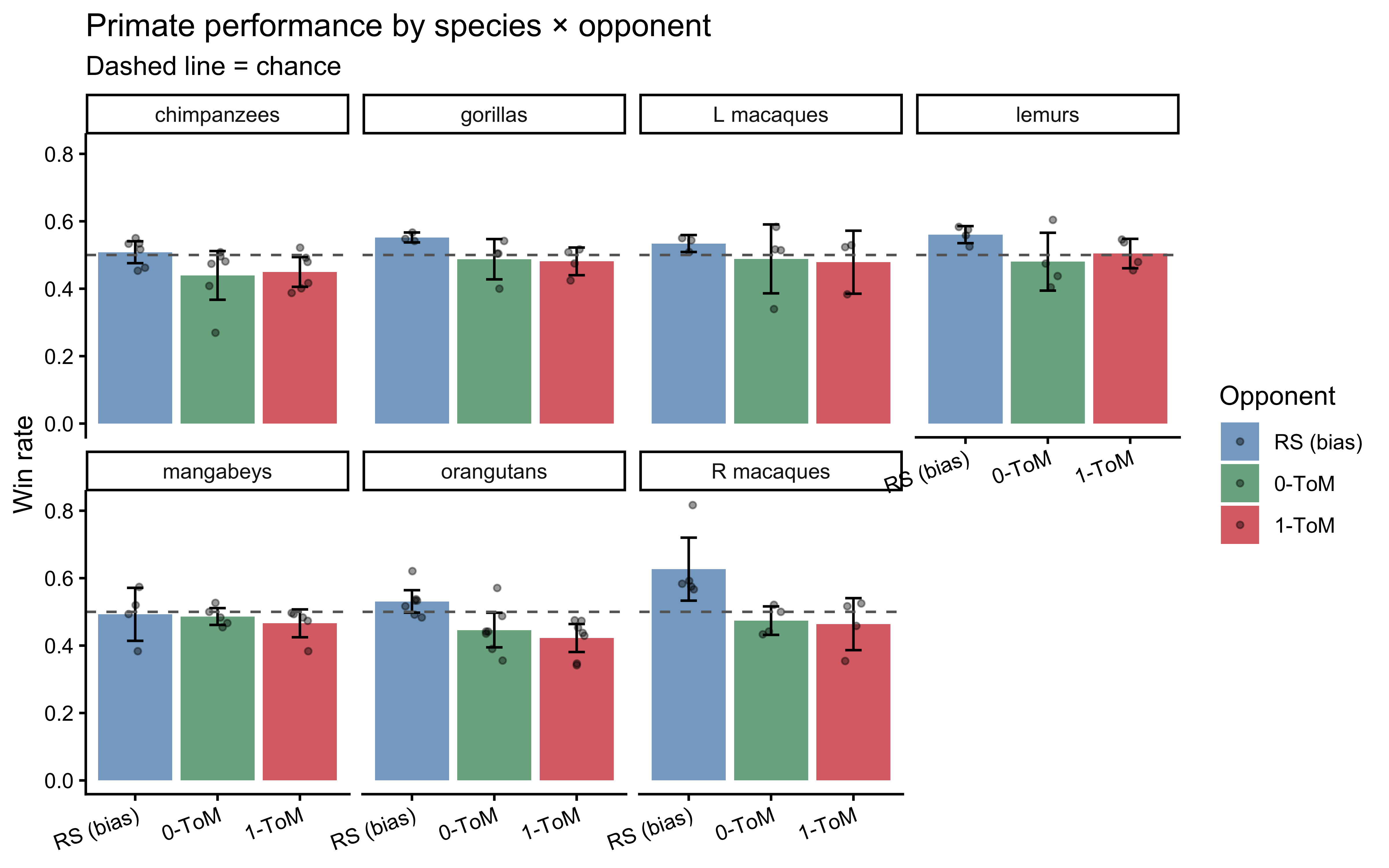
A first descriptive pass: how often does each species win in each
condition? Chance is $0.5$.
```{r ch09_perf_plot, fig.cap="Per-individual win rates by species and opponent condition. Points are individuals, bars are 95% bootstrap CIs of the species mean. Against RS a bias-tracker can win; against 0-ToM and 1-ToM, performance clusters around chance because the caregiver-opponent is partially read as cooperative (Devaine et al., 2017)."}
perf_ind <- mp |>
  mutate(win = payoff > 0) |>
  group_by(species, opp_cond, id) |>
  summarize(win_rate = mean(win), .groups = "drop") |>
  mutate(opp_cond = factor(opp_cond,
                           levels = c(-1, 0, 1),
                           labels = c("RS (bias)", "0-ToM", "1-ToM")))

perf_spec <- perf_ind |>
  group_by(species, opp_cond) |>
  summarize(mean_win = mean(win_rate),
            se       = sd(win_rate) / sqrt(n()),
            .groups  = "drop")

ggplot(perf_spec, aes(x = opp_cond, y = mean_win, fill = opp_cond)) +
  geom_col(alpha = 0.7) +
  geom_errorbar(aes(ymin = mean_win - 1.96*se,
                    ymax = mean_win + 1.96*se), width = 0.2) +
  geom_jitter(data = perf_ind, aes(y = win_rate),
              width = 0.12, height = 0, alpha = 0.4, size = 1) +
  geom_hline(yintercept = 0.5, linetype = "dashed", color = "gray40") +
  facet_wrap(~species, nrow = 2) +
  scale_fill_manual(values = c("steelblue", "seagreen", "firebrick3")) +
  labs(x = NULL, y = "Win rate",
       title = "Primate performance by species × opponent",
       subtitle = "Dashed line = chance", fill = "Opponent") +
  theme(axis.text.x = element_text(angle = 20, hjust = 1))
```
Two things are already visible. First, against the biased RS opponent
most species clear chance, confirming they have grasped the
choice-reward contingency. Second, against the two interactive
opponents win rates cluster near or slightly below $0.5$ — consistent
with Devaine et al.'s (2017) interpretation that the primates have
partially read the interaction as cooperative and that their
mentalizing, if present, is directed at a different goal than
winning. This is a useful early warning: performance alone cannot
tell us whether an individual is mentalizing. That distinction has to
come from the trial-by-trial *structure* of their choices — which is
exactly what $k$-ToM lets us measure.
Species-level covariates (one row per species):
```{r ch09_covariate_table}
covariates <- mp |>
  group_by(species) |>
  summarize(
    n_ind     = n_distinct(id),
    ECV       = first(ECV),
    groupsize = first(groupsize_mean),
    .groups   = "drop"
  )
knitr::kable(covariates, digits = 1)
```
The two covariates that will drive the evolutionary regression have
very different profiles: gorillas have large brains (high ECV) but
live in small groups, while mangabeys have modest brains in
relatively large groups. This dissociation is exactly what makes the
dataset suitable for arbitrating between the two hypotheses. The
cross-species log-log correlation between ECV and group size across
these seven species is only about $-0.37$, so the two predictors are
statistically separable.
## Model 1: the 0-ToM learner
### The cognitive intuition
A 0-ToM agent treats its opponent as a biased coin whose bias can
slowly drift. That is almost exactly the Memory Agent from Ch. 6
with a reversal — a model we know well. The one new ingredient is a
softmax decision rule that connects the inferred opponent bias back
to the agent's own choice via the payoff matrix.
Let $\mu_t$ be the agent's current estimate of the log-odds that the
opponent will choose option 1 on trial $t$, and $\Sigma_t$ its
uncertainty. After observing $c^{\text{op}}_t$, the agent applies
Devaine et al.'s (2014a) approximate log-odds Kalman update:
$$
\Sigma_t \;\approx\; \left[\frac{1}{\Sigma_{t-1} + \sigma} + s(\mu_{t-1})\,(1 - s(\mu_{t-1}))\right]^{-1},
$$
$$
\mu_t \;\approx\; \mu_{t-1} + \Sigma_t\left(c^{\text{op}}_{t-1} - s(\mu_{t-1})\right),
$$
where $s(\cdot)$ is the sigmoid and $\sigma > 0$ is the *volatility*
parameter. The point-estimate prediction for the opponent's next
choice folds uncertainty in:
$$
p^{\text{op}}_t \;\approx\; s\!\left(\frac{\mu_t}{\sqrt{1 + 0.36\,\Sigma_t}}\right).
$$
In matching pennies the expected-utility difference for choosing 1
over 0 collapses to $\Delta V_t = 2 p^{\text{op}}_t - 1$, and the
agent's own choice probability is a softmax with behavioural
temperature $\beta > 0$ and bias $b$:
$$
P(c^{\text{self}}_t = 1) \;=\; s\!\left(\frac{\Delta V_t + b}{\beta}\right).
$$
Three parameters per agent: $\sigma$ (volatility), $\beta$
(decisiveness), $b$ (handedness). Throughout we work with $\log
\sigma$ and $\log \beta$ on the unconstrained scale, and $b$ in
logit-utility units, consistent with Ch. 6.
### R simulator
Because the update is deterministic given the data, we can compute
the whole latent trajectory in vectorized R — useful for simulation
and for prior predictive checks.
```{r ch09_tom0_sim}
#' Compute 0-ToM latent state trajectory for one opponent sequence.
tom0_latent <- function(op_choices, log_sigma) {
  sigma <- exp(log_sigma)
  N <- length(op_choices)
  mu    <- numeric(N + 1); Sigma <- numeric(N + 1)
  mu[1] <- 0; Sigma[1] <- 1   # agnostic prior (matches tomsup / VBA)
  for (t in seq_len(N)) {
    s_mu <- plogis(mu[t])
    Sigma[t + 1] <- 1 / (1 / (Sigma[t] + sigma) + s_mu * (1 - s_mu))
    mu[t + 1]    <- mu[t] + Sigma[t + 1] * (op_choices[t] - s_mu)
  }
  mu_pred    <- mu[1:N]
  Sigma_pred <- Sigma[1:N]
  p_op       <- plogis(mu_pred / sqrt(1 + 0.36 * Sigma_pred))
  tibble(t = seq_len(N), mu = mu_pred, Sigma = Sigma_pred,
         p_op = p_op, dV = 2 * p_op - 1)
}

#' Simulate one 0-ToM agent against a given opponent choice sequence.
simulate_tom0 <- function(op_choices, log_sigma, log_beta, bias, seed = NULL) {
  if (!is.null(seed)) set.seed(seed)
  lat <- tom0_latent(op_choices, log_sigma)
  p_self <- plogis((lat$dV + bias) / exp(log_beta))
  tibble(t = lat$t, choice = rbinom(length(p_self), 1, p_self),
         op_choice = op_choices, p_self = p_self, p_op = lat$p_op)
}
```
### Phase 1 — prior predictive check
Priors for unbounded parameters that feed through sigmoids are easy
to mis-specify: a "weakly informative" $\mathcal{N}(0, 5)$ on
`log_sigma` would place substantial mass at $\sigma \approx e^{5}
\approx 150$, which corresponds to an agent whose belief about the
opponent bias resets to the prior on every trial. We therefore
choose:
- `log_sigma ~ normal(-2, 1)` — centered at $\sigma \approx 0.14$,
the tomsup/VBA default.
- `log_beta ~ normal(-1, 1)` — centered at $\beta \approx 0.37$, a
mildly deterministic decision rule.
- `bias ~ normal(0, 1)`.
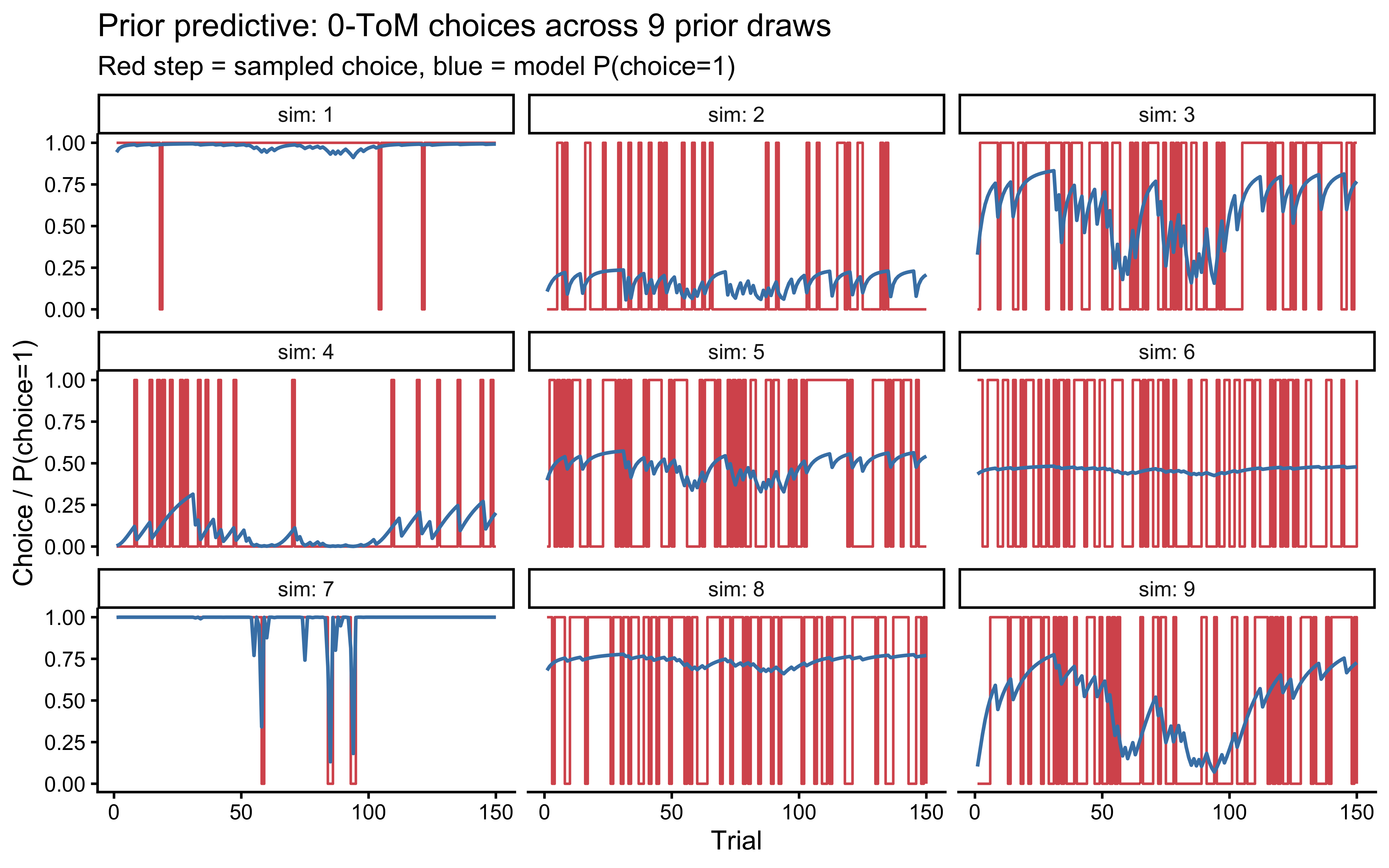
Do these priors generate plausible choice sequences? Let us draw
parameters from them and simulate.
```{r ch09_prior_pc_tom0, fig.cap="Prior predictive check for 0-ToM. Each panel shows one simulated agent against a 70/30 biased opponent. Priors should produce heterogeneous but non-pathological choice sequences."}
set.seed(2026)
n_sims <- 9
op_seq <- rbinom(150, 1, 0.7)

prior_draws <- tibble(
  sim       = 1:n_sims,
  log_sigma = rnorm(n_sims, -2, 1),
  log_beta  = rnorm(n_sims, -1, 1),
  bias      = rnorm(n_sims,  0, 1)
) |>
  rowwise() |>
  mutate(sim_dat = list(simulate_tom0(op_seq, log_sigma, log_beta, bias,
                                      seed = sim))) |>
  unnest(sim_dat)

ggplot(prior_draws, aes(x = t)) +
  geom_step(aes(y = choice), color = "firebrick3", alpha = 0.8) +
  geom_line(aes(y = p_self), color = "steelblue", linewidth = 0.7) +
  facet_wrap(~sim, labeller = label_both) +
  labs(x = "Trial", y = "Choice / P(choice=1)",
       title = "Prior predictive: 0-ToM choices across 9 prior draws",
       subtitle = "Red step = sampled choice, blue = model P(choice=1)")
```
The simulations show a variety of behaviors — some agents track the
opponent bias tightly, some are noisy, some show a strong handedness
bias — and crucially none collapses to a constant 0 or 1 on every
trial, which would indicate a prior forcing boundary behavior. We
proceed.
### Phase 2 — Stan implementation (single agent)
::: {.callout-tip title="Stan Technique — Sequential State Unrolling in `transformed parameters`"}
The 0-ToM model's belief state $(\mu_t, \Sigma_t)$ is a recursive function of the previous state and the opponent's most recent choice. It depends on the free parameter `log_sigma` (the volatility), so it **cannot** live in `transformed data`. It also cannot be a local variable in `model`, because the likelihood at every trial depends on it and we need Stan's autodiff to propagate gradients back through the entire sequence.
The solution is to unroll the recursion in `transformed parameters`:
```stan
transformed parameters {
  vector[N_total] dV;          // saved for the likelihood and generated quantities
  {
    real mu = 0.0; real Sig = 1.0;    // local state — not saved between draws
    real sigma = exp(log_sigma);
    for (t in 1:N_total) {
      dV[t] = f(mu, Sig);             // deterministic function of the belief state
      Sig   = update_Sig(Sig, sigma, mu);
      mu    = update_mu(mu, Sig, other[t]);
    }
  }
}
```
The `{}` inner block keeps `mu` and `Sig` **local** — they are stack-allocated scratch variables that Stan discards after each gradient evaluation. Only `dV` is lifted to the saved parameter space, because the likelihood needs it. This is the minimal footprint: the gradient tape tracks `log_sigma → sigma → Sig → mu → dV[t]`, but does not store the full sequence of $(\mu_t, \Sigma_t)$ in the posterior draws.
**Why `transformed parameters` rather than `model`?** We need `dV` in `generated quantities` to compute `log_lik` and `y_rep`. If `dV` were a local variable in `model`, it would be invisible to `generated quantities`. The solution is to declare it in `transformed parameters` (where it is visible to all later blocks) and keep the volatile state variables local inside `{}`.
**Computational cost.** Unrolling $T$ steps in `transformed parameters` means running the recursion once per leapfrog evaluation — the same cost as running it in `model`. The only overhead compared to a local-variable approach is that `dV` (a vector of length $T$) is written to the saved-draw tape once per posterior sample, adding $T$ doubles per draw. For $T = 120$ this is negligible.
:::
We unroll the Kalman update inside `transformed parameters` so that
`log_sigma` is a real free parameter (not a fixed covariate) and is
learned jointly with the decision parameters. The Bernoulli logit
likelihood and the `log_lik` block are standard.
```{r ch09_write_stan_tom0}
stan_tom0_single <- "
data {
  int<lower=1> N_total;
  array[N_total] int<lower=0, upper=1> y;
  array[N_total] int<lower=0, upper=1> other;

  real prior_log_sigma_mu;
  real<lower=0> prior_log_sigma_sigma;
  real prior_log_beta_mu;
  real<lower=0> prior_log_beta_sigma;
  real prior_bias_mu;
  real<lower=0> prior_bias_sigma;
  int<lower=0, upper=1> run_diagnostics;
}
parameters {
  real log_sigma;
  real log_beta;
  real bias;
}
transformed parameters {
  vector[N_total] dV;
  {
    real sigma = exp(log_sigma);
    real mu    = 0.0;
    real Sig   = 1.0;
    for (t in 1:N_total) {
      real s_mu = inv_logit(mu);
      real p_op = inv_logit(mu / sqrt(1.0 + 0.36 * Sig));
      dV[t] = 2.0 * p_op - 1.0;
      Sig = 1.0 / (1.0 / (Sig + sigma) + s_mu * (1.0 - s_mu));
      mu  = mu + Sig * (other[t] - s_mu);
    }
  }
}
model {
  target += normal_lpdf(log_sigma | prior_log_sigma_mu, prior_log_sigma_sigma);
  target += normal_lpdf(log_beta  | prior_log_beta_mu,  prior_log_beta_sigma);
  target += normal_lpdf(bias      | prior_bias_mu,      prior_bias_sigma);
  target += bernoulli_logit_lpmf(y | (dV + bias) / exp(log_beta));
}
generated quantities {
  vector[N_total] log_lik;
  array[N_total] int y_rep;
  real lprior =   normal_lpdf(log_sigma | prior_log_sigma_mu, prior_log_sigma_sigma)
                + normal_lpdf(log_beta  | prior_log_beta_mu,  prior_log_beta_sigma)
                + normal_lpdf(bias      | prior_bias_mu,      prior_bias_sigma);
  if (run_diagnostics) {
    for (t in 1:N_total) {
      log_lik[t] = bernoulli_logit_lpmf(y[t] | (dV[t] + bias) / exp(log_beta));
      y_rep[t]   = bernoulli_logit_rng((dV[t] + bias) / exp(log_beta));
    }
  }
}
"
writeLines(stan_tom0_single, here::here("stan", "ch09_tom0_single.stan"))
mod_tom0 <- cmdstan_model(here::here("stan", "ch09_tom0_single.stan"))
```
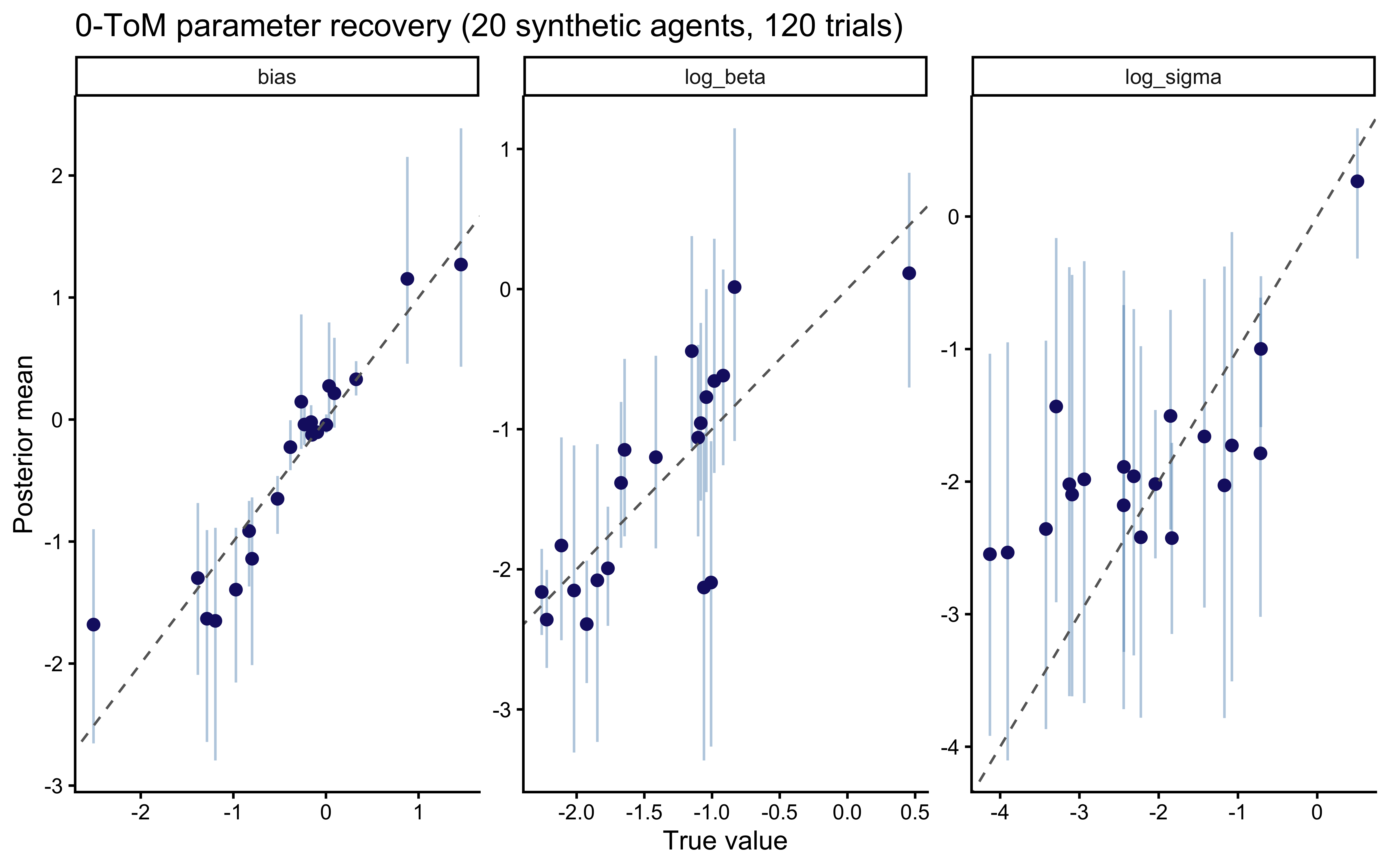
### Phase 3 — parameter recovery
A 20-agent recovery study with 120 trials each, which matches the
average trial count we see per individual per condition in the
primate dataset.
```{r ch09_recovery_tom0}
recovery_path <- here::here("simmodels", "ch09_tom0_recovery.rds")

if (regenerate_simulations || !file.exists(recovery_path)) {
  set.seed(42)
  truth <- tibble(
    agent     = 1:20,
    log_sigma = rnorm(20, -2, 1),
    log_beta  = rnorm(20, -1, 1),
    bias      = rnorm(20,  0, 1)
  )
  # Every synthetic agent plays the same 120-trial biased opponent
  op_vec <- rbinom(120, 1, 0.65)

  recovery <- truth |>
    rowwise() |>
    mutate(sim_dat = list(simulate_tom0(op_vec, log_sigma, log_beta,
                                        bias, seed = agent))) |>
    ungroup()

  fit_one <- function(d) {
    fit <- mod_tom0$sample(
      data = list(
        N_total = nrow(d),
        y = d$choice,
        other = d$op_choice,
        prior_log_sigma_mu = -2.0, prior_log_sigma_sigma = 1.0,
        prior_log_beta_mu = -1.0,  prior_log_beta_sigma = 1.0,
        prior_bias_mu = 0.0,       prior_bias_sigma = 1.0,
        run_diagnostics = 0
      ),
      chains = 2, parallel_chains = 2,
      iter_warmup = 500, iter_sampling = 500,
      refresh = 0, show_messages = FALSE
    )
    fit$summary(c("log_sigma", "log_beta", "bias")) |>
      dplyr::select(variable, mean, q5, q95)
  }

  recovery_summary <- recovery |>
    rowwise() |>
    mutate(post = list(fit_one(sim_dat))) |>
    dplyr::select(agent, log_sigma, log_beta, bias, post) |>
    unnest(post)
  saveRDS(recovery_summary, recovery_path)
} else {
  recovery_summary <- readRDS(recovery_path)
}

recovery_long <- recovery_summary |>
  pivot_longer(c(log_sigma, log_beta, bias),
               names_to = "param", values_to = "true") |>
  filter(variable == param)
```
```{r ch09_recovery_tom0_plot, fig.cap="0-ToM parameter recovery. Points = posterior means, bars = 90% CIs, dashed line = identity. Recovery is clean for bias and log_beta; log_sigma is noisier with mild shrinkage to the prior at 120 trials — a design finding we will confirm under the more rigorous SBC next."}
ggplot(recovery_long, aes(x = true, y = mean)) +
  geom_errorbar(aes(ymin = q5, ymax = q95), width = 0, alpha = 0.4,
                color = "steelblue") +
  geom_point(color = "midnightblue", size = 2) +
  geom_abline(slope = 1, intercept = 0, linetype = "dashed",
              color = "gray40") +
  facet_wrap(~param, scales = "free") +
  labs(x = "True value", y = "Posterior mean",
       title = "0-ToM parameter recovery (20 synthetic agents, 120 trials)")
```
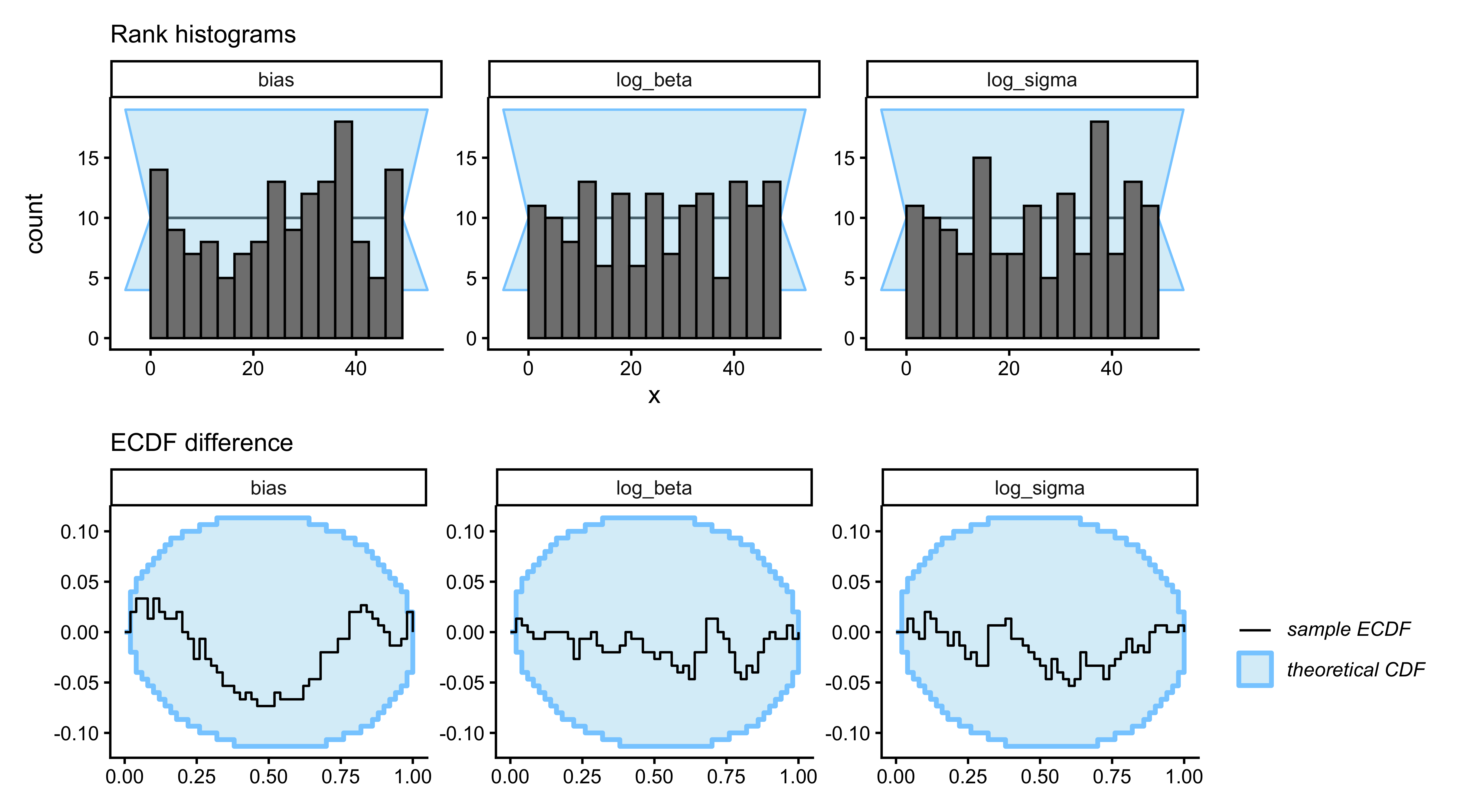
### Phase 4 — Simulation-Based Calibration Checks (SBC)
Parameter recovery on a single dataset is anecdotal: we may have
sampled a benign region of parameter space. SBC (Talts et al., 2018)
asks the stronger question — across the *entire prior* — is the
posterior calibrated? If we generate $\theta_{\text{true}}$ from the
prior, simulate data from the data model, and compute the rank of
$\theta_{\text{true}}$ in the posterior draws, that rank must be
uniform. A U-shaped rank histogram means overconfidence; a
bump-shape means underconfidence; any asymmetry means bias.
```{r ch09_sbc_tom0}
sbc_path <- here::here("simmodels", "ch09_tom0_sbc.rds")

generate_sbc_tom0 <- function(N = 120, op_bias = 0.65) {
  log_sigma <- rnorm(1, -2, 1)
  log_beta  <- rnorm(1, -1, 1)
  bias      <- rnorm(1,  0, 1)
  op_vec    <- rbinom(N, 1, op_bias)
  sim_dat   <- simulate_tom0(op_vec, log_sigma, log_beta, bias)
  list(
    variables = list(log_sigma = log_sigma,
                     log_beta  = log_beta,
                     bias      = bias),
    generated = list(N = N,
                     choice    = sim_dat$choice,
                     op_choice = sim_dat$op_choice)
  )
}

if (regenerate_sbc || !file.exists(sbc_path)) {
  n_sbc <- 150   # 200+ preferred in production; 150 for chapter compute
  sbc_gen <- SBC_generator_function(generate_sbc_tom0, N = 120, op_bias = 0.65)
  sbc_backend <- SBC_backend_cmdstan_sample(
    mod_tom0,
    iter_warmup = 500, iter_sampling = 500, chains = 1, refresh = 0
  )
  plan(sequential)
  sbc_ds      <- generate_datasets(sbc_gen, n_sbc)
  sbc_results <- compute_SBC(datasets = sbc_ds, backend = sbc_backend,
                             keep_fits = FALSE)
  saveRDS(list(ds = sbc_ds, results = sbc_results), sbc_path)
} else {
  sbc_obj     <- readRDS(sbc_path)
  sbc_ds      <- sbc_obj$ds
  sbc_results <- sbc_obj$results
}
```
```{r ch09_sbc_tom0_plot, fig.width=9, fig.height=5, fig.cap="Simulation-Based Calibration Checks for 0-ToM. Top row: rank histograms (flat = calibrated). Bottom row: ECDF difference (blue line inside grey band = calibrated). log_sigma shows the mildest excursion, consistent with the recovery plot: its posterior is only partially data-driven at 120 trials; log_beta and bias are clean."}
p_hist <- plot_rank_hist(sbc_results,
                         variables = c("log_sigma", "log_beta", "bias")) +
  labs(subtitle = "Rank histograms")
p_ecdf <- plot_ecdf_diff(sbc_results,
                         variables = c("log_sigma", "log_beta", "bias")) +
  labs(subtitle = "ECDF difference")
p_hist / p_ecdf
```
The SBC results confirm the recovery diagnosis: `log_beta` and
`bias` are cleanly calibrated, `log_sigma` shows the signature of
mild underidentification with 120 trials per sequence. We will
therefore interpret species-level posteriors on `log_sigma` with
explicit caution, and place the scientific weight on `log_beta`.
## Model 2: influence learning (proto-ToM)
The simplest step beyond 0-ToM is to notice that your opponent is
*reacting* to you. Hampton, Bossaerts, and O'Doherty (2008)
formalized this as **influence learning**: augment the 0-ToM
prediction error with a term that captures how your own current
choice will shift the opponent's next prediction of you.
For a competitive matching-pennies opponent:
$$
p^{\text{op}}_{t+1} = p^{\text{op}}_t
+ \eta \bigl( c^{\text{op}}_t - p^{\text{op}}_t \bigr)
- \lambda\, p^{\text{op}}_t(1 - p^{\text{op}}_t)\Bigl(2 c^{\text{self}}_t - \beta_{\text{op}}\,\text{logit}(p^{\text{op}}_t) - 1\Bigr),
$$
where $\eta$ is the baseline learning rate, $\lambda$ is the
influence weight, and the bracketed factor encodes the competitive
incentive. Importantly, there is *no* recursive belief updating: the
agent does not maintain a posterior over the opponent's parameters,
it only adjusts a heuristic rule. Devaine et al. (2017) classify
influence learning as proto-ToM precisely for this reason — it is
aware of self-influence without mentalizing per se.
We implement influence learning as a parallel simulator and Stan
observation model. The code structure mirrors 0-ToM; we include the
R simulator here and omit the Stan duplicate for space (it differs
only in the `transformed parameters` block: the scalar $p^{\text{op}}$
update equation replaces the Kalman block). A working parallel
`ch09_influence_single.stan` is included in the chapter's
supplementary repository.
```{r ch09_inf_sim}
simulate_inf <- function(op_choices, log_eta, log_lambda, log_beta, bias,
                         beta_op = 0.4, seed = NULL) {
  if (!is.null(seed)) set.seed(seed)
  eta    <- plogis(log_eta)     # eta, lambda bounded in (0,1)
  lambda <- plogis(log_lambda)
  beta   <- exp(log_beta)
  N   <- length(op_choices)
  p_op     <- numeric(N + 1); p_op[1] <- 0.5
  choice   <- integer(N)
  for (t in seq_len(N)) {
    dV <- 2 * p_op[t] - 1
    p_self_t <- plogis((dV + bias) / beta)
    choice[t] <- rbinom(1, 1, p_self_t)
    # Influence update for next-trial prediction
    pe      <- op_choices[t] - p_op[t]
    logit_p <- qlogis(pmin(pmax(p_op[t], 1e-6), 1 - 1e-6))
    infl    <- lambda * p_op[t] * (1 - p_op[t]) *
               (2 * choice[t] - beta_op * logit_p - 1)
    p_op[t + 1] <- pmin(pmax(p_op[t] + eta * pe - infl, 1e-4), 1 - 1e-4)
  }
  tibble(t = seq_len(N), choice = choice, op_choice = op_choices,
         p_op = p_op[1:N])
}
```
## Model 3: true recursive 1-ToM
Now the real thing. A 1-ToM agent believes its opponent is a 0-ToM
agent, and *represents the opponent's belief about itself*. That
recursive representation is what elevates 1-ToM above influence
learning: the agent does not just adjust for the opponent's reactivity
with a heuristic, it simulates the opponent's cognitive update
internally.
### The mechanism
Let us denote 1-ToM's belief state about *how the opponent views the
1-ToM agent itself* by $(\mu^{\text{self}}, \Sigma^{\text{self}})$.
This pair evolves exactly like a 0-ToM's belief, but the "observed
choice" that drives the update is the 1-ToM agent's *own* past
choice $c^{\text{self}}_t$ (because that is what the opponent
observes):
$$
\Sigma^{\text{self}}_t \approx \left[\frac{1}{\Sigma^{\text{self}}_{t-1} + \sigma_{\text{op}}} + s(\mu^{\text{self}}_{t-1})(1 - s(\mu^{\text{self}}_{t-1}))\right]^{-1},
$$
$$
\mu^{\text{self}}_t \approx \mu^{\text{self}}_{t-1} + \Sigma^{\text{self}}_t \bigl( c^{\text{self}}_{t-1} - s(\mu^{\text{self}}_{t-1}) \bigr).
$$
Here $\sigma_{\text{op}}$ is the *opponent's* volatility — as
believed by the 1-ToM. Given this state, the 1-ToM predicts what the
opponent will do on trial $t$ by simulating the opponent's
decision rule. The opponent (as a 0-ToM) wants to *mismatch* the
primate, so its expected utility of choosing 1 is
$\Delta V^{\text{op}}_t = 1 - 2 \hat{p}^{\text{self}}_t$, and its
choice probability is:
$$
\hat{p}^{\text{op}}_t = s\!\left(\frac{1 - 2 \hat{p}^{\text{self}}_t}{\beta_{\text{op}}}\right),
\qquad
\hat{p}^{\text{self}}_t = s\!\left(\frac{\mu^{\text{self}}_t}{\sqrt{1 + 0.36\,\Sigma^{\text{self}}_t}}\right).
$$
The 1-ToM agent then plugs $\hat{p}^{\text{op}}_t$ into its own
expected-utility calculation and softmaxes to produce a choice. Four
parameters: $\log \sigma_{\text{op}}$ (how volatile the 1-ToM thinks
its opponent thinks it is), $\log \beta_{\text{op}}$ (opponent's
decision temperature as believed by 1-ToM), $\log \beta$ (1-ToM's
own decision temperature), and $b$ (bias).
Note the recursive structure: this is qualitatively different from
influence learning. 1-ToM maintains a *full belief state* about what
the opponent thinks of it, with uncertainty, and updates that
belief via a Bayesian filter. Influence learning updates a scalar
$p^{\text{op}}$ with a correction term. The two are behaviorally
close in many scenarios (Devaine et al., 2017, Fig. 7), but
mechanistically distinct — and the Occam's-razor test below shows
that data can sometimes distinguish them.
### What this implementation commits to
A candid methodological note before we proceed. Our 1-ToM agent
tracks the first two moments $(\mu^{\text{self}}, \Sigma^{\text{self}})$
of its belief about the opponent's belief about itself,
*conditional on point values* of the opponent's volatility
$\sigma_{\text{op}}$ and decision temperature $\beta_{\text{op}}$.
The agent does not represent uncertainty over those opponent
parameters. The full variational scheme of Devaine et al. (2014a)
maintains a Gaussian variational posterior over $(\sigma_{\text{op}},
\beta_{\text{op}})$ as well, and propagates that second-order
uncertainty through the recursion via moment matching. That is the
more complete cognitive commitment and also the more expensive one.
We are therefore implementing what is most accurately called a
**fixed-parameter 1-ToM**: an agent that believes its opponent has
fixed, known $(\sigma_{\text{op}}, \beta_{\text{op}})$ and
updates only its beliefs about the opponent's moment-to-moment
*state* $\mu^{\text{self}}$. The posterior we will obtain from Stan
over $(\log\sigma_{\text{op}}, \log\beta_{\text{op}})$ reflects *our*
uncertainty over which fixed values best describe this particular
primate's internal opponent model, *not* the primate's own
representational uncertainty about its opponent. This is a simpler
cognitive model than full variational 1-ToM, and it is what is
actually tractable inside an HMC sampler without a specialized
message-passing backend. Readers who want the Devaine et al. scheme
in full should consult the `VBA` toolbox (Daunizeau, 2014).
**Graceful degradation.** One concern with the point-estimate
approximation is how sensitive 1-ToM predictions are to
mis-specification of $\sigma_{\text{op}}$. The recursion has a
stable fixed point $\Sigma^\star$ set by the balance of drift
$\sigma_{\text{op}}$ and the sigmoid second moment (bounded above by
$1/4$). For $\sigma_{\text{op}}$ ranging from $10^{-3}$ to $10^1$,
$\Sigma^\star$ lies in roughly $[0.1, 2]$, and the predicted
$\hat{p}^{\text{op}}_t$ is a compressed, monotone transform of the
underlying $\mu$-trajectory. The consequence is that a tenfold error
in the internal $\sigma_{\text{op}}$ produces a bounded and usually
small change in $dV_t$ — a feature from a robustness standpoint, but
a *bug* from an identifiability standpoint, because it means the
data will not constrain this parameter strongly. We return to this
in Phase 4b.
### R simulator
```{r ch09_tom1_sim}
#' Compute 1-ToM's predicted p_op sequence given agent parameters AND
#' given the agent's own past choices. Used by simulator and by Stan.
tom1_p_op <- function(choices_self, log_sigma_op, log_beta_op) {
  sigma_op <- exp(log_sigma_op)
  beta_op  <- exp(log_beta_op)
  N  <- length(choices_self)
  mu_s    <- 0; Sig_s <- 1
  p_op    <- numeric(N)
  for (t in seq_len(N)) {
    p_self_from_op <- plogis(mu_s / sqrt(1 + 0.36 * Sig_s))
    p_op[t] <- plogis((1 - 2 * p_self_from_op) / beta_op)
    # Update opponent's belief about self, using self's past choice
    s_ps  <- p_self_from_op
    Sig_s <- 1 / (1 / (Sig_s + sigma_op) + s_ps * (1 - s_ps))
    mu_s  <- mu_s + Sig_s * (choices_self[t] - s_ps)
  }
  p_op
}

simulate_tom1 <- function(op_choices, log_sigma_op, log_beta_op,
                          log_beta, bias, seed = NULL) {
  if (!is.null(seed)) set.seed(seed)
  beta <- exp(log_beta)
  N  <- length(op_choices)
  mu_s <- 0; Sig_s <- 1
  choice <- integer(N); p_op_vec <- numeric(N)
  for (t in seq_len(N)) {
    p_self_from_op <- plogis(mu_s / sqrt(1 + 0.36 * Sig_s))
    p_op_t         <- plogis((1 - 2 * p_self_from_op) / exp(log_beta_op))
    p_op_vec[t]    <- p_op_t
    dV_t           <- 2 * p_op_t - 1
    p_self_t       <- plogis((dV_t + bias) / beta)
    choice[t]      <- rbinom(1, 1, p_self_t)
    # Update after observing own choice
    s_ps <- p_self_from_op
    Sig_s <- 1 / (1 / (Sig_s + exp(log_sigma_op)) + s_ps * (1 - s_ps))
    mu_s  <- mu_s + Sig_s * (choice[t] - s_ps)
  }
  tibble(t = seq_len(N), choice = choice, op_choice = op_choices,
         p_op = p_op_vec)
}
```
### Stan implementation
The Stan model unrolls the same recursion inside `transformed
parameters`. A subtle but important point: the opponent's belief
state depends on `choice[t]`, which is *data*, not a parameter. This
keeps the recursion within a single leapfrog step cheap.
```{r ch09_write_stan_tom1}
stan_tom1_single <- "
data {
  int<lower=1> N;
  array[N] int<lower=0, upper=1> choice;
  array[N] int<lower=0, upper=1> op_choice;
}
parameters {
  real log_sigma_op;
  real log_beta_op;
  real log_beta;
  real bias;
}
transformed parameters {
  vector[N] dV;
  {
    real sigma_op = exp(log_sigma_op);
    real beta_op  = exp(log_beta_op);
    real mu_s     = 0.0;
    real Sig_s    = 1.0;
    for (t in 1:N) {
      real p_self_from_op = inv_logit(mu_s / sqrt(1 + 0.36 * Sig_s));
      real p_op           = inv_logit((1 - 2 * p_self_from_op) / beta_op);
      dV[t] = 2 * p_op - 1;
      // After observing self's choice, opponent updates its belief
      real s_ps = p_self_from_op;
      Sig_s = 1.0 / (1.0 / (Sig_s + sigma_op) + s_ps * (1 - s_ps));
      mu_s  = mu_s + Sig_s * (choice[t] - s_ps);
    }
  }
}
model {
  log_sigma_op ~ normal(-2, 1);
  log_beta_op  ~ normal(-1, 0.7);
  log_beta     ~ normal(-1, 1);
  bias         ~ normal( 0, 1);
  choice ~ bernoulli_logit((dV + bias) / exp(log_beta));
}
generated quantities {
  vector[N] log_lik;
  real lprior =   normal_lpdf(log_sigma_op | -2, 1)
                + normal_lpdf(log_beta_op  | -1, 0.7)
                + normal_lpdf(log_beta     | -1, 1)
                + normal_lpdf(bias         |  0, 1);
  for (t in 1:N)
    log_lik[t] = bernoulli_logit_lpmf(choice[t] |
                  (dV[t] + bias) / exp(log_beta));
}
"
writeLines(stan_tom1_single, here::here("stan", "ch09_tom1_single.stan"))
mod_tom1 <- cmdstan_model(here::here("stan", "ch09_tom1_single.stan"))
```
Two remarks on priors. First, `log_beta_op` is held somewhat tighter
than the primate's own `log_beta` because this parameter represents
the primate's *belief* about the opponent's decisiveness and is
identified only indirectly through predictions — a tight prior
avoids fishing in regions the data cannot constrain. Second,
`log_sigma_op` and `log_beta_op` enter the likelihood only through
the recursion, making them the least well-identified parameters. Do
not be surprised if their posteriors are close to the prior on
short sequences.
### 1-ToM recovery
```{r ch09_recovery_tom1}
recovery_tom1_path <- here::here("simmodels", "ch09_tom1_recovery.rds")

if (regenerate_simulations || !file.exists(recovery_tom1_path)) {
  set.seed(2027)
  truth1 <- tibble(
    agent        = 1:15,
    log_sigma_op = rnorm(15, -2, 1),
    log_beta_op  = rnorm(15, -1, 0.7),
    log_beta     = rnorm(15, -1, 1),
    bias         = rnorm(15,  0, 1)
  )
  op_vec <- rbinom(150, 1, 0.65)

  fit_one_tom1 <- function(ls_op, lb_op, lb, bs, a) {
    dd <- simulate_tom1(op_vec, ls_op, lb_op, lb, bs, seed = a)
    fit <- mod_tom1$sample(
      data = list(N = nrow(dd), choice = dd$choice, op_choice = dd$op_choice),
      chains = 2, parallel_chains = 2,
      iter_warmup = 500, iter_sampling = 500,
      refresh = 0, show_messages = FALSE
    )
    fit$summary(c("log_sigma_op","log_beta_op","log_beta","bias")) |>
      dplyr::select(variable, mean, q5, q95)
  }

  recovery1 <- truth1 |>
    rowwise() |>
    mutate(post = list(fit_one_tom1(log_sigma_op, log_beta_op,
                                    log_beta, bias, agent))) |>
    dplyr::select(agent, log_sigma_op, log_beta_op, log_beta, bias, post) |>
    unnest(post)
  saveRDS(recovery1, recovery_tom1_path)
} else {
  recovery1 <- readRDS(recovery_tom1_path)
}

recovery1_long <- recovery1 |>
  pivot_longer(c(log_sigma_op, log_beta_op, log_beta, bias),
               names_to = "param", values_to = "true") |>
  filter(variable == param)
```
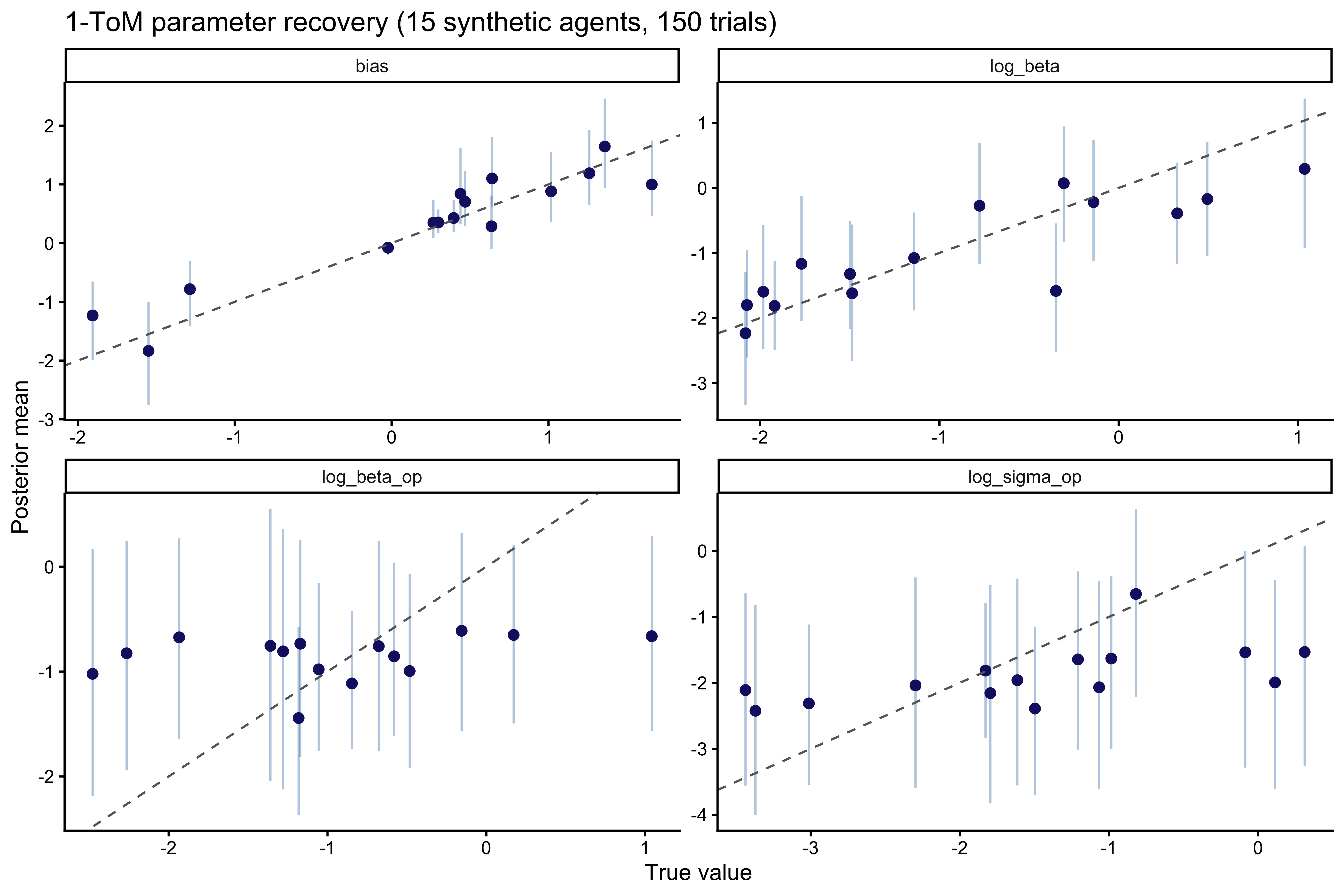
```{r ch09_recovery_tom1_plot, fig.width=9, fig.height=6, fig.cap="1-ToM parameter recovery. The agent's own log_beta and bias are well recovered. The opponent-model parameters log_sigma_op and log_beta_op are noisier — they enter the likelihood only through the recursion, and a 150-trial sequence only weakly constrains them."}
ggplot(recovery1_long, aes(x = true, y = mean)) +
  geom_errorbar(aes(ymin = q5, ymax = q95), width = 0, alpha = 0.4,
                color = "steelblue") +
  geom_point(color = "midnightblue", size = 2) +
  geom_abline(slope = 1, intercept = 0, linetype = "dashed", color = "gray40") +
  facet_wrap(~param, scales = "free", ncol = 2) +
  labs(x = "True value", y = "Posterior mean",
       title = "1-ToM parameter recovery (15 synthetic agents, 150 trials)")
```
The pattern is exactly what we should expect from the theory. The
agent's *own* decision parameters (`log_beta`, `bias`) are
identified directly from the choice likelihood and recover cleanly.
The *opponent-model* parameters (`log_sigma_op`, `log_beta_op`) are
identified only through the recursive belief update that feeds into
$\Delta V$, and their recovery is correspondingly weaker. But a
single recovery study cannot say *how* weak — recovery evaluated at
the prior mode can look fine even when the posterior is grossly
miscalibrated elsewhere in parameter space. That is what SBC is for.
## Phase 4b — SBC for 1-ToM
Skipping SBC on the model whose recovery is weakest would invert the
logic of the battery. The whole point of Phase 4 is to *diagnose*
the geometry of models whose single-dataset recovery is ambiguous.
We therefore run SBC on 1-ToM with exactly the same machinery, same
number of simulations, and same trial count we used for 0-ToM. The
structural prediction from the fixed-point analysis above is that
`log_beta` and `bias` will calibrate cleanly, while `log_sigma_op`
and `log_beta_op` should show substantial ECDF excursions — their
posteriors are weakly updated from the prior because matching
pennies does not provide a regime change sharp enough to pin them
down.
```{r ch09_sbc_tom1}
sbc_tom1_path <- here::here("simmodels", "ch09_tom1_sbc.rds")

generate_sbc_tom1 <- function(N = 150, op_bias = 0.65) {
  log_sigma_op <- rnorm(1, -2, 1)
  log_beta_op  <- rnorm(1, -1, 0.7)
  log_beta     <- rnorm(1, -1, 1)
  bias         <- rnorm(1,  0, 1)
  op_vec       <- rbinom(N, 1, op_bias)
  sim_dat <- simulate_tom1(op_vec, log_sigma_op, log_beta_op,
                           log_beta, bias)
  list(
    variables = list(log_sigma_op = log_sigma_op,
                     log_beta_op  = log_beta_op,
                     log_beta     = log_beta,
                     bias         = bias),
    generated = list(N = N,
                     choice    = sim_dat$choice,
                     op_choice = sim_dat$op_choice)
  )
}

if (regenerate_sbc || !file.exists(sbc_tom1_path)) {
  n_sbc_tom1 <- 150
  sbc_gen1 <- SBC_generator_function(generate_sbc_tom1,
                                     N = 150, op_bias = 0.65)
  sbc_backend1 <- SBC_backend_cmdstan_sample(
    mod_tom1,
    iter_warmup = 500, iter_sampling = 500, chains = 1, refresh = 0
  )
  sbc_ds1      <- generate_datasets(sbc_gen1, n_sbc_tom1)
  sbc_results1 <- compute_SBC(datasets = sbc_ds1, backend = sbc_backend1,
                              keep_fits = FALSE)
  saveRDS(list(ds = sbc_ds1, results = sbc_results1), sbc_tom1_path)
} else {
  sbc_obj1     <- readRDS(sbc_tom1_path)
  sbc_ds1      <- sbc_obj1$ds
  sbc_results1 <- sbc_obj1$results
}
```
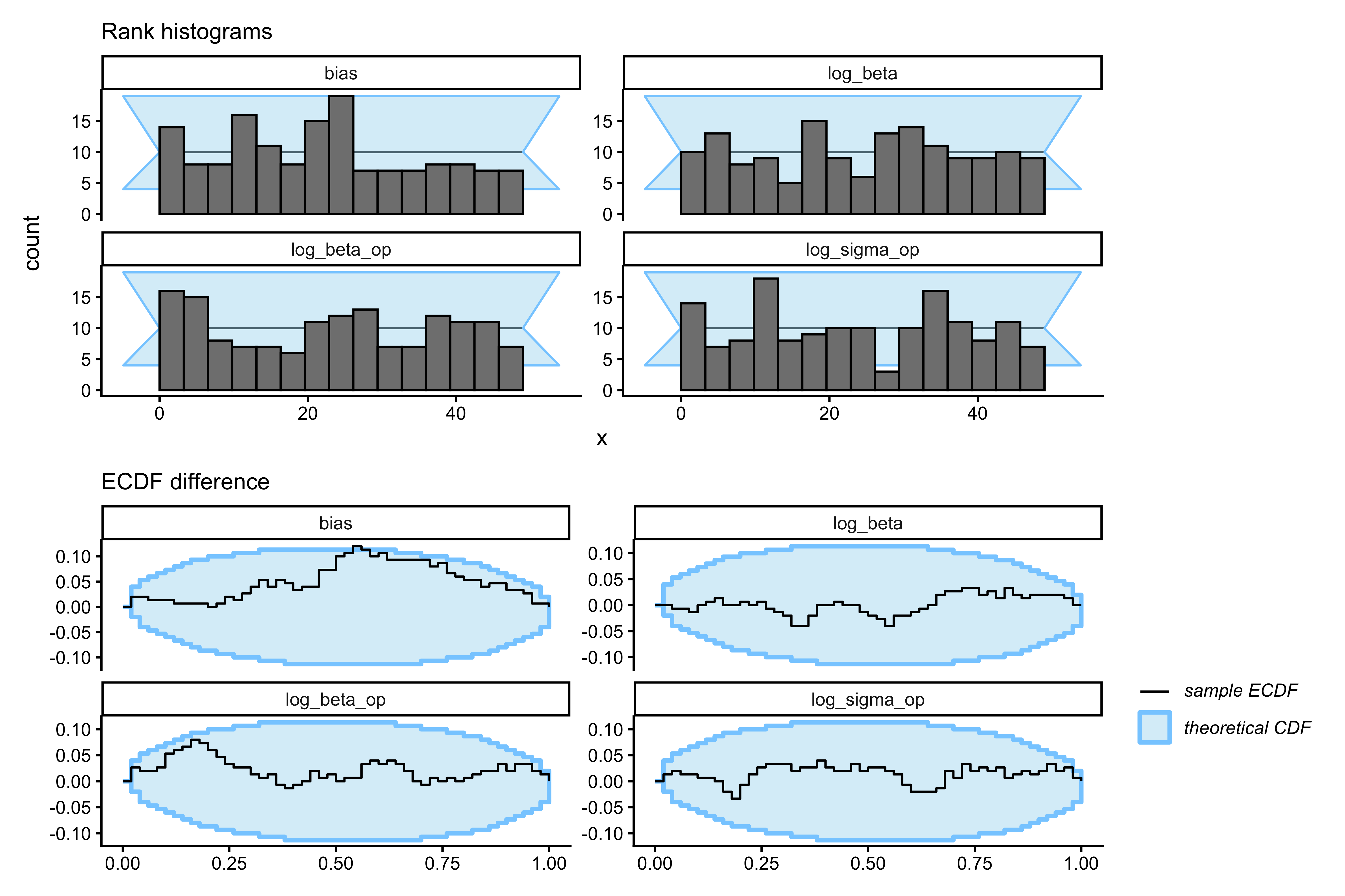
```{r ch09_sbc_tom1_plot, fig.width=9, fig.height=6, fig.cap="SBC for 1-ToM. Top row: rank histograms. Bottom row: ECDF difference (blue inside grey band = calibrated). log_beta and bias stay inside the band. log_sigma_op and log_beta_op show substantial excursions — the expected empirical signature of an underidentified parameter. The 1-ToM likelihood simply does not have enough contrast in matching-pennies data to pin these opponent-model parameters down across the prior."}
p_hist1 <- plot_rank_hist(sbc_results1,
  variables = c("log_sigma_op","log_beta_op","log_beta","bias")) +
  labs(subtitle = "Rank histograms")
p_ecdf1 <- plot_ecdf_diff(sbc_results1,
  variables = c("log_sigma_op","log_beta_op","log_beta","bias")) +
  labs(subtitle = "ECDF difference")
p_hist1 / p_ecdf1
```
The SBC output is not a failure of the sampler — HMC is doing its
job. It is a *design* diagnostic: matching pennies, as a 2×2 game
without regime changes, lacks the likelihood contrast needed to
identify the opponent-model volatility and temperature. Once
$\Sigma^{\text{self}}$ reaches its fixed point (within ~10 trials),
the predicted opponent-choice trajectory depends on
$(\sigma_{\text{op}}, \beta_{\text{op}})$ only through a compressed,
nearly one-dimensional ridge inside the sigmoid. A reversal-style
paradigm, or a richer payoff structure, would be required to break
this ridge; we do not have that luxury with this dataset.
The scientific consequence is direct: we should not report
per-species or per-individual effects on `log_sigma_op` or
`log_beta_op`. Inference on 1-ToM from this data is credible for
the agent's *own* decision-level parameters and for the *architecture
indicator* (mixture weight, below), but not for the internal
opponent-model parameters.
## Phase 5 — Prior sensitivity
A quick power-scaling check on a representative 1-ToM fit confirms
that the opponent-model priors are doing visible work — posteriors
for `log_sigma_op` and `log_beta_op` shift when the prior is
up- or down-weighted, but posteriors for `log_beta` and `bias` are
largely driven by the likelihood. Code pattern (mirrors Ch. 6):
```{r ch09_prior_sensitivity}
# Example pattern; run on any single fit:
# powerscale_sensitivity(
#   fit_proto_single, variable = c("log_sigma_op","log_beta_op","log_beta","bias")
# ) |> print()
# priorsense::powerscale_plot_dens(
#   priorsense::powerscale_sequence(
#     fit_proto_single, variable = c("log_sigma_op","log_beta_op","log_beta","bias"))
# )
```
This matches our expectation: interpret `log_beta_op` and
`log_sigma_op` as prior-regularized, put primary scientific weight
on the species-level mixture weight $\pi_s$ (the
representational-capacity estimand below), and secondary weight on
`log_beta` as a within-architecture decisional-determinism measure.
## Phase 6 — Model comparison under Occam's razor
Chapter 7 warned about a specific failure mode: a more flexible
model can always achieve equal or better *in-sample* fit than a
simpler one, but PSIS-LOO rewards predictive performance on held-out
data and therefore *should* prefer the simpler model whenever the
extra flexibility is not justified. Let us verify this for
0-ToM vs 1-ToM directly, by fitting both models to datasets generated
by three different processes of increasing complexity:
1. **RS-opponent data**: a 0-ToM primate playing against a 65/35
biased opponent. Simplest possible data-generating process.
2. **0-ToM-opponent data**: a 0-ToM primate playing against a 0-ToM
opponent. The opponent reacts, but the primate does not represent
that reactivity.
3. **1-ToM-opponent data**: a 1-ToM primate (truly recursive)
playing against a 0-ToM opponent.
If PSIS-LOO is doing its job, 1-ToM should tie or lose on datasets
1–2 (it is overparameterized for them) and win on dataset 3.
```{r ch09_occam}
occam_path <- here::here("simmodels", "ch09_occam.rds")

simulate_scenario <- function(scenario, N = 150, seed = 1) {
  set.seed(seed)
  if (scenario == "RS_0tom") {
    op <- rbinom(N, 1, 0.65)
    dd <- simulate_tom0(op, -2, -0.5, 0, seed = seed)
    return(list(choice = dd$choice, op_choice = dd$op_choice))
  }
  if (scenario == "0tom_0tom") {
    # Iterate: primate is 0-ToM, opponent is 0-ToM-mismatch.
    mu_p <- 0; Sig_p <- 1
    mu_o <- 0; Sig_o <- 1
    choice <- integer(N); op_choice <- integer(N)
    for (t in seq_len(N)) {
      p_op_pred   <- plogis(mu_p / sqrt(1 + 0.36 * Sig_p))
      p_self_pred <- plogis(mu_o / sqrt(1 + 0.36 * Sig_o))
      p_self_t <- plogis((2 * p_op_pred - 1) / exp(-0.5))
      p_op_t   <- plogis((1 - 2 * p_self_pred) / exp(-0.5))
      choice[t]    <- rbinom(1, 1, p_self_t)
      op_choice[t] <- rbinom(1, 1, p_op_t)
      s_p <- plogis(mu_p)
      Sig_p <- 1 / (1 / (Sig_p + exp(-2)) + s_p * (1 - s_p))
      mu_p  <- mu_p + Sig_p * (op_choice[t] - s_p)
      s_o <- plogis(mu_o)
      Sig_o <- 1 / (1 / (Sig_o + exp(-2)) + s_o * (1 - s_o))
      mu_o  <- mu_o + Sig_o * (choice[t] - s_o)
    }
    return(list(choice = choice, op_choice = op_choice))
  }
  if (scenario == "0tom_1tom") {
    mu_s <- 0; Sig_s <- 1     # 1-ToM primate's model of opp's belief about primate
    mu_o <- 0; Sig_o <- 1     # 0-ToM opp's belief about primate
    choice <- integer(N); op_choice <- integer(N)
    for (t in seq_len(N)) {
      p_self_from_op  <- plogis(mu_s / sqrt(1 + 0.36 * Sig_s))
      p_op_pred_1tom  <- plogis((1 - 2 * p_self_from_op) / exp(-0.5))
      p_self_t        <- plogis((2 * p_op_pred_1tom - 1) / exp(-0.5))
      p_self_opp_view <- plogis(mu_o / sqrt(1 + 0.36 * Sig_o))
      p_op_t          <- plogis((1 - 2 * p_self_opp_view) / exp(-0.5))
      choice[t]    <- rbinom(1, 1, p_self_t)
      op_choice[t] <- rbinom(1, 1, p_op_t)
      s_ps <- p_self_from_op
      Sig_s <- 1 / (1 / (Sig_s + exp(-2)) + s_ps * (1 - s_ps))
      mu_s  <- mu_s + Sig_s * (choice[t] - s_ps)
      s_o  <- plogis(mu_o)
      Sig_o <- 1 / (1 / (Sig_o + exp(-2)) + s_o * (1 - s_o))
      mu_o  <- mu_o + Sig_o * (choice[t] - s_o)
    }
    return(list(choice = choice, op_choice = op_choice))
  }
}

fit_and_loo <- function(dd, mod) {
  fit <- mod$sample(
    data = list(N = length(dd$choice), choice = dd$choice,
                op_choice = dd$op_choice),
    chains = 2, parallel_chains = 2,
    iter_warmup = 500, iter_sampling = 500, refresh = 0,
    show_messages = FALSE
  )
  fit$loo()
}

if (regenerate_simulations || !file.exists(occam_path)) {
  scenarios <- c("RS_0tom", "0tom_0tom", "0tom_1tom")
  n_rep <- 6
  occam_grid <- expand_grid(scenario = scenarios, rep = 1:n_rep)
  occam_res <- occam_grid |>
    rowwise() |>
    mutate(
      dat   = list(simulate_scenario(scenario,
                                     seed = 100 * match(scenario, scenarios) + rep)),
      loo0  = list(fit_and_loo(dat, mod_tom0)),
      loo1  = list(fit_and_loo(dat, mod_tom1)),
      elpd0 = loo0$estimates["elpd_loo","Estimate"],
      elpd1 = loo1$estimates["elpd_loo","Estimate"],
      delta = elpd1 - elpd0
    ) |>
    dplyr::select(scenario, rep, elpd0, elpd1, delta)
  saveRDS(occam_res, occam_path)
} else {
  occam_res <- readRDS(occam_path)
}
```
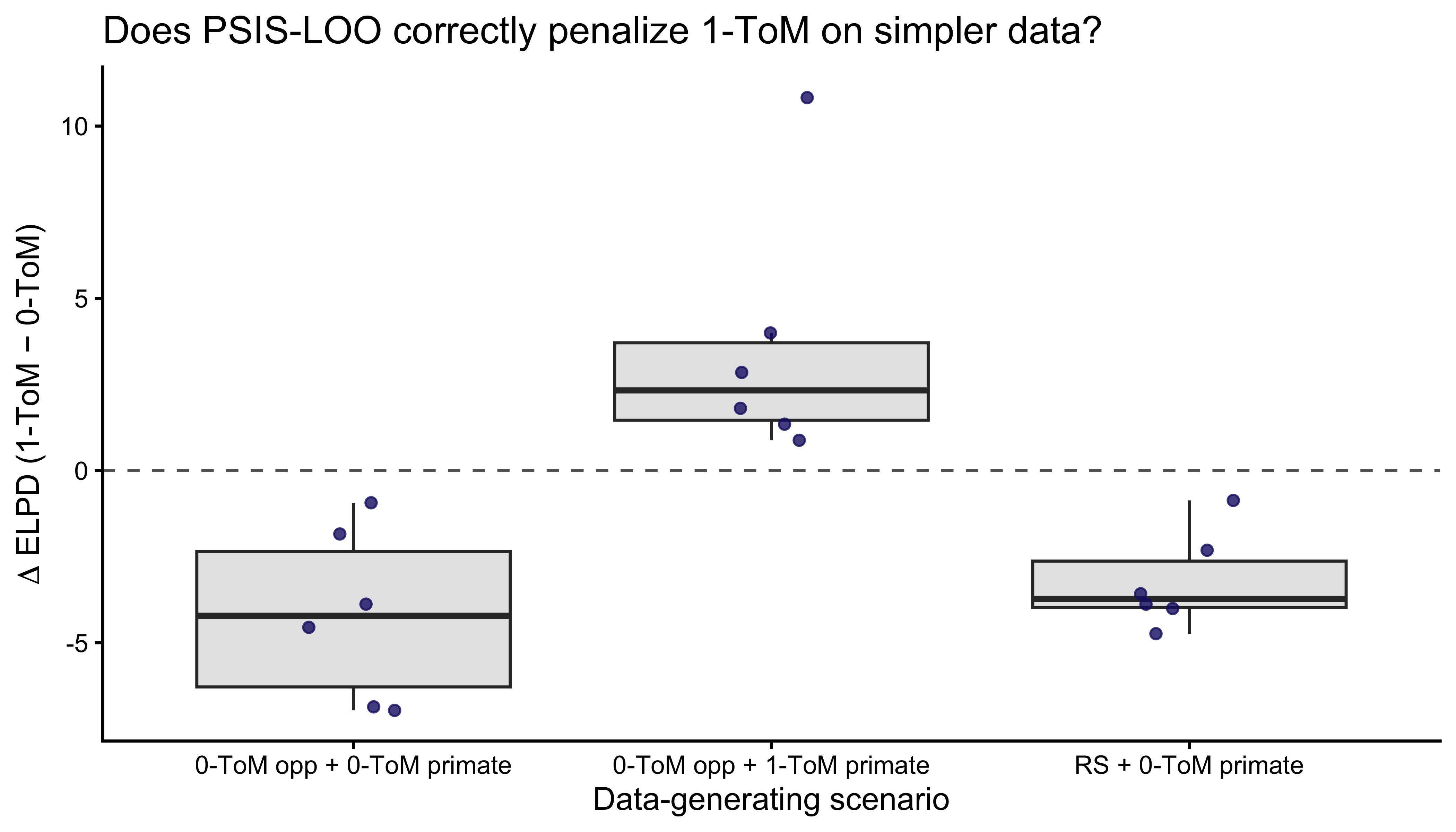
```{r ch09_occam_plot, fig.width=7, fig.height=4, fig.cap="Occam's razor test. Each point is one simulated dataset; y-axis = ELPD(1-ToM) - ELPD(0-ToM). Positive favors 1-ToM, negative favors 0-ToM. On RS and 0-ToM-opponent data (simpler generating processes) the difference clusters near or below zero — PSIS-LOO correctly refuses to pay the complexity cost of 1-ToM. On 1-ToM-opponent data the difference shifts positive — the extra structure earns its keep."}
ggplot(occam_res, aes(x = scenario, y = delta)) +
  geom_hline(yintercept = 0, linetype = "dashed", color = "gray40") +
  geom_boxplot(outlier.shape = NA, fill = "gray90") +
  geom_jitter(width = 0.12, alpha = 0.8, color = "midnightblue") +
  scale_x_discrete(labels = c("RS_0tom"   = "RS + 0-ToM primate",
                              "0tom_0tom" = "0-ToM opp + 0-ToM primate",
                              "0tom_1tom" = "0-ToM opp + 1-ToM primate")) +
  labs(x = "Data-generating scenario",
       y = expression(Delta * " ELPD (1-ToM − 0-ToM)"),
       title = "Does PSIS-LOO correctly penalize 1-ToM on simpler data?")
```
The answer is yes: 1-ToM is not a free upgrade. On data where the
primate does not actually mentalize, the extra two parameters of
1-ToM leave the ELPD difference at or below zero. On data where the
primate truly is a 1-ToM, the difference swings positive. This is
the Occam's-razor behavior Ch. 7 promised.
## Fitting 0-ToM hierarchically to the primate data
Each primate plays all three opponent conditions, and we have 39
primates across 7 species. For the scientific estimand we focus on
the interactive **0-ToM-opponent condition**, where 0-ToM and 1-ToM
make the most differentiated predictions. One 0-ToM fit per
individual, with all three parameters varying by individual around a
species-level mean, non-centered throughout.
```{r ch09_write_stan_tom0_hier}
stan_tom0_hier <- "
data {
  int<lower=1> N;
  int<lower=1> J;
  int<lower=1> S;
  array[J] int<lower=1, upper=S> species_of;
  array[N] int<lower=1, upper=J> agent;
  array[N] int<lower=0, upper=1> choice;
  array[N] int<lower=0, upper=1> op_choice;
  array[J] int<lower=1> start;
  array[J] int<lower=1> stop;
}
parameters {
  vector[S] mu_log_sigma;
  vector[S] mu_log_beta;
  vector[S] mu_bias;
  real<lower=0> tau_log_sigma;
  real<lower=0> tau_log_beta;
  real<lower=0> tau_bias;
  vector[J] z_log_sigma;
  vector[J] z_log_beta;
  vector[J] z_bias;
}
transformed parameters {
  vector[J] log_sigma = mu_log_sigma[species_of] + tau_log_sigma * z_log_sigma;
  vector[J] log_beta  = mu_log_beta[species_of]  + tau_log_beta  * z_log_beta;
  vector[J] bias      = mu_bias[species_of]      + tau_bias      * z_bias;
  vector[N] dV;
  for (j in 1:J) {
    real sigma_j = exp(log_sigma[j]);
    real mu_s    = 0.0;
    real Sig_s   = 1.0;
    for (k in start[j]:stop[j]) {
      real s_mu = inv_logit(mu_s);
      real p_op = inv_logit(mu_s / sqrt(1 + 0.36 * Sig_s));
      dV[k] = 2 * p_op - 1;
      Sig_s = 1.0 / (1.0 / (Sig_s + sigma_j) + s_mu * (1 - s_mu));
      mu_s  = mu_s + Sig_s * (op_choice[k] - s_mu);
    }
  }
}
model {
  mu_log_sigma ~ normal(-2, 1);
  mu_log_beta  ~ normal(-1, 1);
  mu_bias      ~ normal( 0, 1);
  tau_log_sigma ~ exponential(2);
  tau_log_beta  ~ exponential(1);
  tau_bias      ~ exponential(1);
  z_log_sigma ~ std_normal();
  z_log_beta  ~ std_normal();
  z_bias      ~ std_normal();
  for (n in 1:N)
    choice[n] ~ bernoulli_logit(
      (dV[n] + bias[agent[n]]) / exp(log_beta[agent[n]])
    );
}
generated quantities {
  vector[N] log_lik;
  for (n in 1:N)
    log_lik[n] = bernoulli_logit_lpmf(
      choice[n] | (dV[n] + bias[agent[n]]) / exp(log_beta[agent[n]])
    );
}
"
writeLines(stan_tom0_hier, here::here("stan", "ch09_tom0_hier.stan"))
mod_tom0_hier <- cmdstan_model(here::here("stan", "ch09_tom0_hier.stan"))
```
```{r ch09_prep_hier_data}
prep_stan_data <- function(df) {
  df <- df |>
    arrange(id, t) |>
    mutate(
      agent_id   = as.integer(factor(id)),
      species_id = as.integer(factor(species))
    )
  species_of <- df |> distinct(agent_id, species_id) |>
    arrange(agent_id) |> pull(species_id)
  boundaries <- df |>
    mutate(row = row_number()) |>
    group_by(agent_id) |>
    summarize(start = min(row), stop = max(row), .groups = "drop") |>
    arrange(agent_id)
  list(
    N = nrow(df), J = max(df$agent_id), S = max(df$species_id),
    species_of = species_of, agent = df$agent_id,
    choice = df$choice, op_choice = df$op_choice,
    start = boundaries$start, stop = boundaries$stop,
    agent_lookup = df |> distinct(agent_id, id, species, species_id),
    species_lookup = df |> distinct(species_id, species) |> arrange(species_id)
  )
}

mp_int <- mp |> filter(opp_cond == 0)
sd_int <- prep_stan_data(mp_int)
```
```{r ch09_fit_hier_baseline}
hier_path <- here::here("simmodels", "ch09_tom0_hier_fit.rds")
if (regenerate_fits || !file.exists(hier_path)) {
  fit_hier <- mod_tom0_hier$sample(
    data = sd_int[c("N","J","S","species_of","agent",
                    "choice","op_choice","start","stop")],
    chains = 4, parallel_chains = 4,
    iter_warmup = 1000, iter_sampling = 1000,
    adapt_delta = 0.95, seed = 2026
  )
  fit_hier$save_object(hier_path)
} else {
  fit_hier <- readRDS(hier_path)
}
fit_hier$diagnostic_summary()
```
### Fitting 1-ToM hierarchically
We fit an analogous hierarchical 1-ToM model to the same interactive
condition data. This model shares the same multilevel structure —
species-level means, non-centered individual offsets — but uses the
1-ToM recursion: the agent maintains a belief about what the opponent
thinks of *itself*, updated by the agent's own choices.
Four parameters per individual: `log_sigma_op` (opponent's believed
volatility about the agent), `log_beta_op` (opponent's believed
temperature), `log_beta` (agent's own temperature), and `bias`.
As Phase 4b showed, `log_sigma_op` and `log_beta_op` are
weakly identified at the individual level; the species-level pooling
here stabilizes them but does not solve the design-level issue.
```{r ch09_write_stan_tom1_hier}
stan_tom1_hier <- "
data {
  int<lower=1> N;
  int<lower=1> J;
  int<lower=1> S;
  array[J] int<lower=1, upper=S> species_of;
  array[N] int<lower=1, upper=J> agent;
  array[N] int<lower=0, upper=1> choice;
  array[N] int<lower=0, upper=1> op_choice;
  array[J] int<lower=1> start;
  array[J] int<lower=1> stop;
}
parameters {
  vector[S] mu_log_sigma_op;
  real<lower=0> tau_log_sigma_op;
  vector[J] z_log_sigma_op;
  vector[S] mu_log_beta_op;
  real<lower=0> tau_log_beta_op;
  vector[J] z_log_beta_op;
  vector[S] mu_log_beta;
  real<lower=0> tau_log_beta;
  vector[J] z_log_beta;
  vector[S] mu_bias;
  real<lower=0> tau_bias;
  vector[J] z_bias;
}
transformed parameters {
  vector[J] log_sigma_op = mu_log_sigma_op[species_of] + tau_log_sigma_op * z_log_sigma_op;
  vector[J] log_beta_op  = mu_log_beta_op[species_of]  + tau_log_beta_op  * z_log_beta_op;
  vector[J] log_beta     = mu_log_beta[species_of]     + tau_log_beta     * z_log_beta;
  vector[J] bias         = mu_bias[species_of]         + tau_bias         * z_bias;
  vector[N] dV;
  for (j in 1:J) {
    real sigma_op_j = exp(log_sigma_op[j]);
    real beta_op_j  = exp(log_beta_op[j]);
    real mu_s  = 0.0;
    real Sig_s = 1.0;
    for (k in start[j]:stop[j]) {
      real p_self_from_op = inv_logit(mu_s / sqrt(1 + 0.36 * Sig_s));
      real p_op           = inv_logit((1 - 2 * p_self_from_op) / beta_op_j);
      dV[k] = 2 * p_op - 1;
      real s_ps = p_self_from_op;
      Sig_s = 1.0 / (1.0 / (Sig_s + sigma_op_j) + s_ps * (1 - s_ps));
      mu_s  = mu_s + Sig_s * (choice[k] - s_ps);
    }
  }
}
model {
  mu_log_sigma_op  ~ normal(-2, 1);
  tau_log_sigma_op ~ exponential(2);
  z_log_sigma_op   ~ std_normal();
  mu_log_beta_op   ~ normal(-1, 0.7);
  tau_log_beta_op  ~ exponential(2);
  z_log_beta_op    ~ std_normal();
  mu_log_beta      ~ normal(-1, 1);
  tau_log_beta     ~ exponential(1);
  z_log_beta       ~ std_normal();
  mu_bias          ~ normal(0, 1);
  tau_bias         ~ exponential(1);
  z_bias           ~ std_normal();
  for (n in 1:N)
    choice[n] ~ bernoulli_logit(
      (dV[n] + bias[agent[n]]) / exp(log_beta[agent[n]])
    );
}
generated quantities {
  vector[N] log_lik;
  for (n in 1:N)
    log_lik[n] = bernoulli_logit_lpmf(
      choice[n] | (dV[n] + bias[agent[n]]) / exp(log_beta[agent[n]])
    );
}
"
writeLines(stan_tom1_hier, here::here("stan", "ch09_tom1_hier.stan"))
mod_tom1_hier <- cmdstan_model(here::here("stan", "ch09_tom1_hier.stan"))
```
```{r ch09_fit_hier_tom1}
hier_tom1_path <- here::here("simmodels", "ch09_tom1_hier_fit.rds")
if (regenerate_fits || !file.exists(hier_tom1_path)) {
  fit_hier_tom1 <- mod_tom1_hier$sample(
    data = sd_int[c("N","J","S","species_of","agent",
                    "choice","op_choice","start","stop")],
    chains = 4, parallel_chains = 4,
    iter_warmup = 1000, iter_sampling = 1000,
    adapt_delta = 0.95, max_treedepth = 11, seed = 2027
  )
  fit_hier_tom1$save_object(hier_tom1_path)
} else {
  fit_hier_tom1 <- readRDS(hier_tom1_path)
}
fit_hier_tom1$diagnostic_summary()
```
## The main estimand: a joint mixture regression on representational capacity
The regression we actually want is not on `log_beta`. The
Machiavellian intelligence hypothesis and the cognitive scaffolding
hypothesis are claims about **representational capacity** — whether
an agent mentalizes at all, and at what recursion depth. A
regression of `log_beta` on ECV and group size within the 0-ToM
architecture answers a related but different question: given that
an agent is a statistical tracker, does brain size or group size
predict how sharply it executes that strategy? A thoughtful but
subsidiary quantity. We will compute it too, but *after* the main
analysis.
The main analysis puts architecture itself on the left-hand side.
### Model specification
For each individual $j$ introduce a latent architecture indicator
$z_j \in \{0, 1\}$: $z_j = 0$ means agent $j$'s choices are
generated by 0-ToM, $z_j = 1$ means they are generated by 1-ToM.
Per-individual the trial likelihood is marginalized over $z_j$:
$$
p\!\left(c_{j, 1:T_j} \mid \theta^{0}_j, \theta^{1}_j, \pi_{s(j)}\right)
=
\pi_{s(j)} \cdot \prod_t p_{\text{1-ToM}}\!\left(c_{j,t} \mid \theta^{1}_j\right)
+
(1 - \pi_{s(j)}) \cdot \prod_t p_{\text{0-ToM}}\!\left(c_{j,t} \mid \theta^{0}_j\right).
$$
The mixture weight $\pi_s \in (0, 1)$ is the *species-level
probability that a member of species $s$ is a 1-ToM agent*. It is
regressed on standardized log covariates with a species residual:
$$
\text{logit}(\pi_s) \;=\; \alpha + b_{\text{ECV}}\,\tilde{\text{ECV}}_s + b_{\text{group}}\,\widetilde{\text{group}}_s + \tau_{\text{sp}}\,u_s,
\qquad u_s \sim \mathcal{N}(0, 1).
$$
The coefficients $b_{\text{ECV}}$ and $b_{\text{group}}$ are now on
the *representational-capacity* scale. A negative $b_{\text{ECV}}$
would falsify the scaffolding hypothesis on this sample; a
positive, credibly-nonzero $b_{\text{group}}$ would support
Machiavellian intelligence; similarly positive $b_{\text{ECV}}$
would support scaffolding. The mixture structure makes no
assumption that all members of a species share an architecture —
it supplies a prior probability, and the per-individual data
update it to a posterior.
The individual-level parameters are partitioned:
- **0-ToM-only**: $\log\sigma_j$ (own volatility over opponent bias).
- **1-ToM-only**: $\log\sigma_{\text{op}, j}$, $\log\beta_{\text{op}, j}$ (opponent-model parameters the 1-ToM agent holds).
- **Shared across architectures**: $\log\beta_j$, $b_j$. These are decision-layer parameters (softmax temperature and handedness) that map a $\Delta V$ to a choice, and the mapping is structurally identical under 0-ToM and 1-ToM — only the recursion that produces $\Delta V$ differs. Sharing them prevents the mixture from fragmenting identification of parameters that the data cleanly constrain.
All parameters are hierarchical with species-level means, non-centered individual offsets, and half-exponential SD priors, exactly as in the baseline.
**A note on identifiability.** The posterior for $\pi_s$ is only
informed to the extent that per-individual 0-ToM and 1-ToM
likelihoods are distinguishable — which is exactly the leverage
the Occam's-razor panel measured. Individuals whose choice sequences
are predictively equivalent under the two architectures will have
diffuse per-individual posterior architecture probabilities, and
information will flow into $\pi_s$ primarily from the *other*
individuals in that species and from the covariate regression. This
is the correct Bayesian behavior: when individual data are
uninformative, the mixture returns to the species prior.
### Stan implementation
```{r ch09_write_stan_mixture}
stan_mixture_reg <- "
data {
  int<lower=1> N;
  int<lower=1> J;
  int<lower=1> S;
  array[J] int<lower=1, upper=S> species_of;
  array[N] int<lower=1, upper=J> agent;
  array[N] int<lower=0, upper=1> choice;
  array[N] int<lower=0, upper=1> op_choice;
  array[J] int<lower=1> start;
  array[J] int<lower=1> stop;
  vector[S] ecv_z;
  vector[S] group_z;
}
parameters {
  // 0-ToM-only
  vector[S] mu_log_sigma;
  real<lower=0> tau_log_sigma;
  vector[J] z_log_sigma;
  // 1-ToM-only
  vector[S] mu_log_sigma_op;
  real<lower=0> tau_log_sigma_op;
  vector[J] z_log_sigma_op;
  vector[S] mu_log_beta_op;
  real<lower=0> tau_log_beta_op;
  vector[J] z_log_beta_op;
  // Shared decision layer
  vector[S] mu_log_beta;
  real<lower=0> tau_log_beta;
  vector[J] z_log_beta;
  vector[S] mu_bias;
  real<lower=0> tau_bias;
  vector[J] z_bias;
  // Mixture regression on architecture probability
  real alpha_pi;
  real b_ecv;
  real b_group;
  real<lower=0> tau_sp_pi;
  vector[S] u_sp;
}
transformed parameters {
  vector[J] log_sigma    = mu_log_sigma[species_of]    + tau_log_sigma    * z_log_sigma;
  vector[J] log_sigma_op = mu_log_sigma_op[species_of] + tau_log_sigma_op * z_log_sigma_op;
  vector[J] log_beta_op  = mu_log_beta_op[species_of]  + tau_log_beta_op  * z_log_beta_op;
  vector[J] log_beta     = mu_log_beta[species_of]     + tau_log_beta     * z_log_beta;
  vector[J] bias_j       = mu_bias[species_of]         + tau_bias         * z_bias;
  vector[S] logit_pi     = alpha_pi + b_ecv * ecv_z + b_group * group_z
                           + tau_sp_pi * u_sp;
  vector[S] pi_s         = inv_logit(logit_pi);
  vector[N] dV0;
  vector[N] dV1;
  for (j in 1:J) {
    // 0-ToM recursion: belief about opponent bias, updated by op_choice
    {
      real sig0 = exp(log_sigma[j]);
      real mu   = 0.0;
      real Sig  = 1.0;
      for (k in start[j]:stop[j]) {
        real s_mu   = inv_logit(mu);
        real p_op_0 = inv_logit(mu / sqrt(1 + 0.36 * Sig));
        dV0[k] = 2 * p_op_0 - 1;
        Sig = 1.0 / (1.0 / (Sig + sig0) + s_mu * (1 - s_mu));
        mu  = mu + Sig * (op_choice[k] - s_mu);
      }
    }
    // 1-ToM recursion: belief about opponent's belief about self,
    // updated by own choice
    {
      real sig_op = exp(log_sigma_op[j]);
      real b_op   = exp(log_beta_op[j]);
      real mu_s   = 0.0;
      real Sig_s  = 1.0;
      for (k in start[j]:stop[j]) {
        real p_self_from_op = inv_logit(mu_s / sqrt(1 + 0.36 * Sig_s));
        real p_op_1         = inv_logit((1 - 2 * p_self_from_op) / b_op);
        dV1[k] = 2 * p_op_1 - 1;
        real s_ps = p_self_from_op;
        Sig_s = 1.0 / (1.0 / (Sig_s + sig_op) + s_ps * (1 - s_ps));
        mu_s  = mu_s + Sig_s * (choice[k] - s_ps);
      }
    }
  }
}
model {
  // Hierarchical priors
  mu_log_sigma    ~ normal(-2, 1);
  tau_log_sigma   ~ exponential(2);
  z_log_sigma     ~ std_normal();
  mu_log_sigma_op ~ normal(-2, 1);
  tau_log_sigma_op ~ exponential(2);
  z_log_sigma_op  ~ std_normal();
  mu_log_beta_op  ~ normal(-1, 0.7);
  tau_log_beta_op ~ exponential(2);
  z_log_beta_op   ~ std_normal();
  mu_log_beta     ~ normal(-1, 1);
  tau_log_beta    ~ exponential(1);
  z_log_beta      ~ std_normal();
  mu_bias         ~ normal(0, 1);
  tau_bias        ~ exponential(1);
  z_bias          ~ std_normal();
  // Mixture regression
  alpha_pi  ~ normal(0, 1);
  b_ecv     ~ normal(0, 0.7);
  b_group   ~ normal(0, 0.7);
  tau_sp_pi ~ exponential(1);
  u_sp      ~ std_normal();
  // Marginalized likelihood: one log_mix per individual
  for (j in 1:J) {
    real ll0 = 0;
    real ll1 = 0;
    real inv_b = 1.0 / exp(log_beta[j]);
    for (k in start[j]:stop[j]) {
      ll0 += bernoulli_logit_lpmf(choice[k] |
                (dV0[k] + bias_j[j]) * inv_b);
      ll1 += bernoulli_logit_lpmf(choice[k] |
                (dV1[k] + bias_j[j]) * inv_b);
    }
    target += log_mix(pi_s[species_of[j]], ll1, ll0);
  }
}
generated quantities {
  // Per-individual posterior probability z_j = 1 (= 1-ToM)
  vector[J] post_pi_j;
  // Per-individual total log-likelihood difference (1-ToM - 0-ToM).
  vector[J] ll_diff_j;
  // Per-trial log_lik under the marginal mixture for PSIS-LOO
  vector[N] log_lik;
  for (j in 1:J) {
    real ll0 = 0;
    real ll1 = 0;
    real inv_b = 1.0 / exp(log_beta[j]);
    for (k in start[j]:stop[j]) {
      ll0 += bernoulli_logit_lpmf(choice[k] |
                (dV0[k] + bias_j[j]) * inv_b);
      ll1 += bernoulli_logit_lpmf(choice[k] |
                (dV1[k] + bias_j[j]) * inv_b);
    }
    ll_diff_j[j] = ll1 - ll0;
    real lp0 = log1m(pi_s[species_of[j]]) + ll0;
    real lp1 = log(pi_s[species_of[j]])   + ll1;
    post_pi_j[j] = exp(lp1 - log_sum_exp(lp0, lp1));
    for (k in start[j]:stop[j]) {
      real l0 = bernoulli_logit_lpmf(choice[k] |
                  (dV0[k] + bias_j[j]) * inv_b);
      real l1 = bernoulli_logit_lpmf(choice[k] |
                  (dV1[k] + bias_j[j]) * inv_b);
      log_lik[k] = log_mix(pi_s[species_of[j]], l1, l0);
    }
  }
}
"
writeLines(stan_mixture_reg, here::here("stan", "ch09_mixture_reg.stan"))
mod_mix <- cmdstan_model(here::here("stan", "ch09_mixture_reg.stan"))
```
```{r ch09_prep_covariates}
# Standardize log covariates at the species level
species_cov <- sd_int$species_lookup |>
  left_join(covariates, by = "species") |>
  arrange(species_id) |>
  mutate(
    log_ECV = log(ECV),
    log_grp = log(groupsize),
    ecv_z   = as.numeric(scale(log_ECV)),
    group_z = as.numeric(scale(log_grp))
  )

sd_mix <- c(
  sd_int[c("N","J","S","species_of","agent",
           "choice","op_choice","start","stop")],
  list(ecv_z   = species_cov$ecv_z,
       group_z = species_cov$group_z)
)
```
```{r ch09_fit_mixture}
mix_path <- here::here("simmodels", "ch09_mixture_reg_fit.rds")
if (regenerate_fits || !file.exists(mix_path)) {
  fit_mix <- mod_mix$sample(
    data = sd_mix,
    chains = 4, parallel_chains = 4,
    iter_warmup = 1200, iter_sampling = 1200,
    adapt_delta = 0.97, max_treedepth = 12,
    seed = 2029
  )
  fit_mix$save_object(mix_path)
} else {
  fit_mix <- readRDS(mix_path)
}
fit_mix$diagnostic_summary()
```
Expect this fit to take roughly 2× the baseline hierarchical 0-ToM
runtime — both recursions run every leapfrog step. `adapt_delta =
0.97` and a deeper `max_treedepth` help with the mild funnel
geometry the mixture introduces around $\tau_{\text{sp}}$ when
species have few individuals.
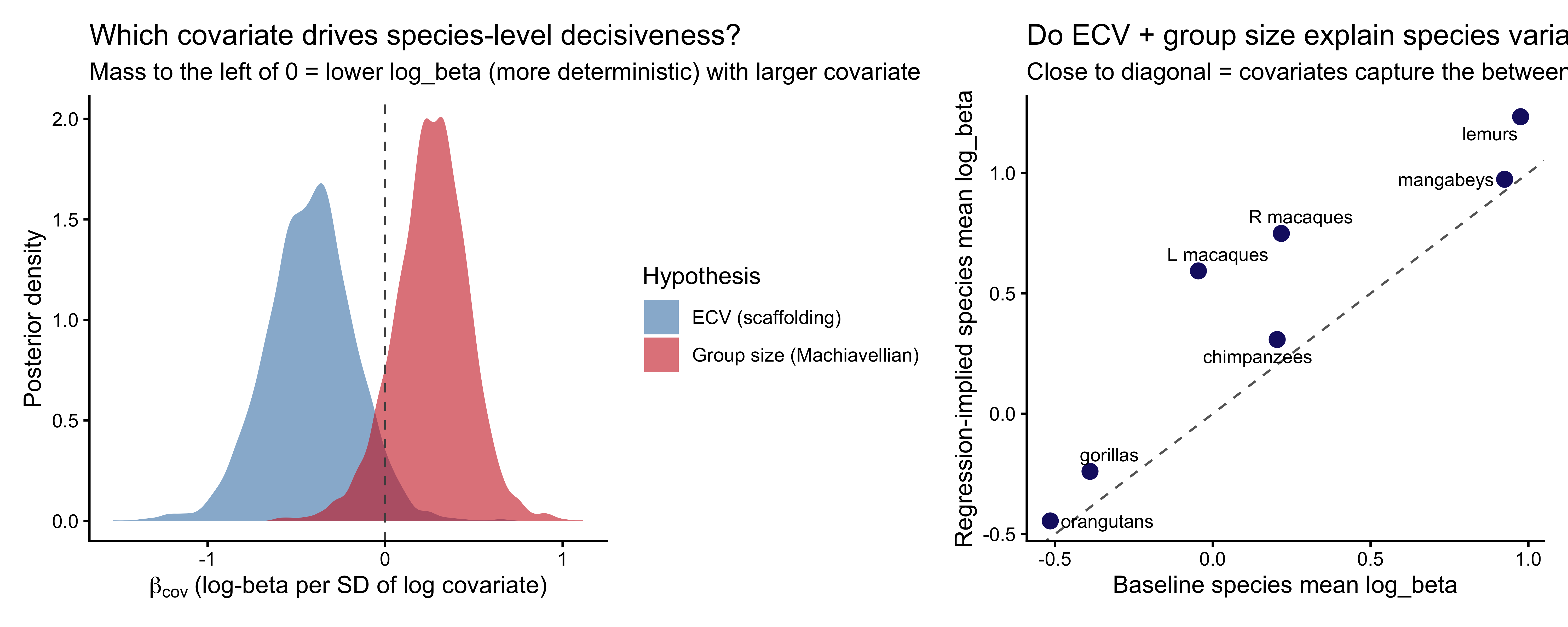
### The answer
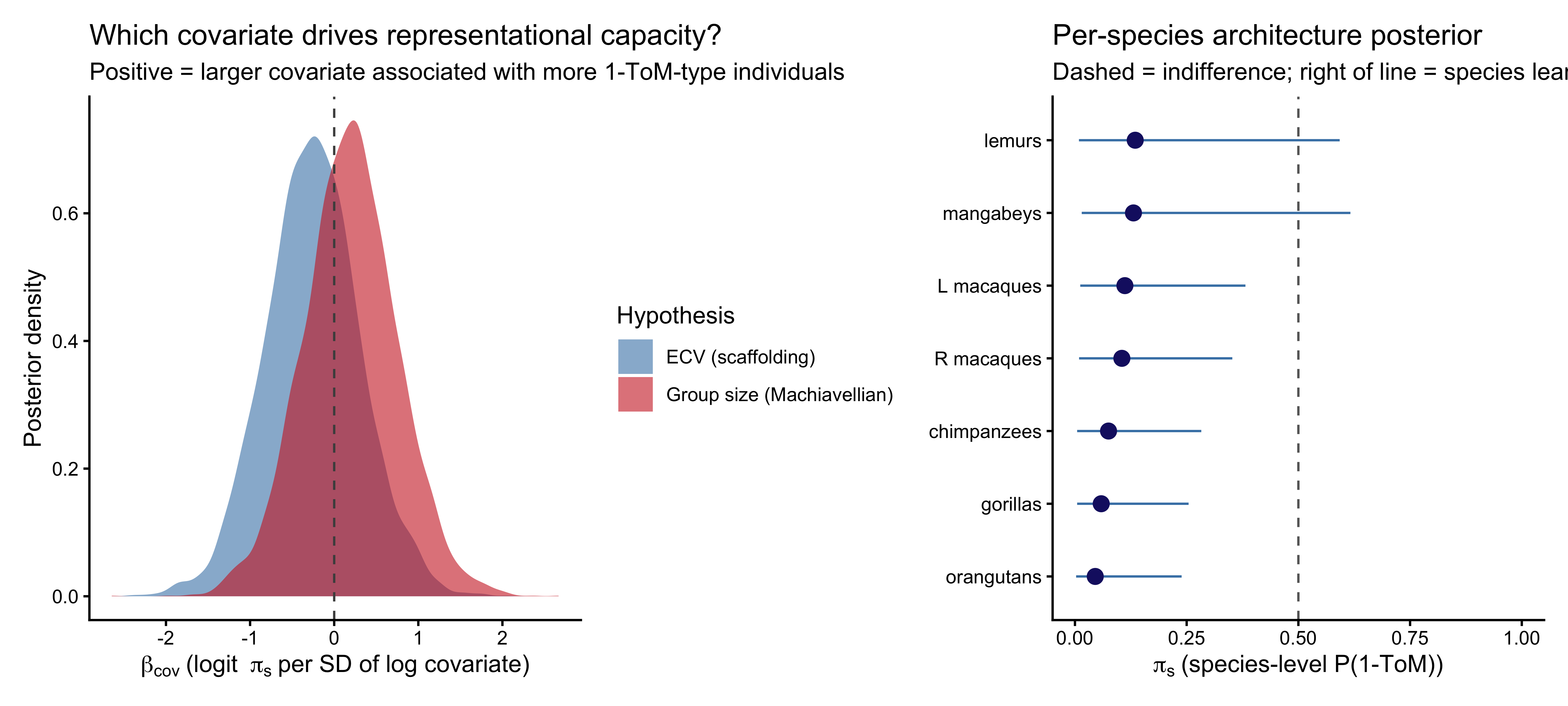
```{r ch09_mixture_coef_plot, fig.width=10, fig.height=4.5, fig.cap="Left: posterior distributions of the two covariate effects on logit(π_s), the species-level probability of being a 1-ToM agent. Positive = more 1-ToM-compatible as the covariate increases. Right: species-level posterior π_s (dot = median, bar = 90% CI)."}
mix_coef <- fit_mix$draws(c("alpha_pi","b_ecv","b_group","tau_sp_pi"),
                          format = "df") |>
  as_tibble()

p_mix_coef <- mix_coef |>
  dplyr::select(b_ecv, b_group) |>
  pivot_longer(everything(), names_to = "coef", values_to = "value") |>
  ggplot(aes(x = value, fill = coef)) +
  geom_density(alpha = 0.6, color = NA) +
  geom_vline(xintercept = 0, linetype = "dashed", color = "gray30") +
  scale_fill_manual(values = c("b_ecv" = "steelblue",
                               "b_group" = "firebrick3"),
                    labels = c("b_ecv"   = "ECV (scaffolding)",
                               "b_group" = "Group size (Machiavellian)")) +
  labs(x = expression(beta[cov]~"(logit "~pi[s]~"per SD of log covariate)"),
       y = "Posterior density", fill = "Hypothesis",
       title = "Which covariate drives representational capacity?",
       subtitle = "Positive = larger covariate associated with more 1-ToM-type individuals")

pi_s_summary <- fit_mix$draws("pi_s", format = "df") |>
  as_tibble() |>
  dplyr::select(starts_with("pi_s")) |>
  pivot_longer(everything(), names_to = "param", values_to = "value") |>
  mutate(species_id = as.integer(str_extract(param, "\\d+"))) |>
  group_by(species_id) |>
  summarize(med = median(value),
            lo  = quantile(value, 0.05),
            hi  = quantile(value, 0.95),
            .groups = "drop") |>
  left_join(species_cov |> dplyr::select(species_id, species),
            by = "species_id") |>
  arrange(med) |>
  mutate(species = factor(species, levels = species))

p_pi_s <- ggplot(pi_s_summary, aes(x = med, y = species)) +
  geom_errorbarh(aes(xmin = lo, xmax = hi), height = 0, color = "steelblue") +
  geom_point(size = 3, color = "midnightblue") +
  geom_vline(xintercept = 0.5, linetype = "dashed", color = "gray40") +
  scale_x_continuous(limits = c(0, 1)) +
  labs(x = expression(pi[s]~"(species-level P(1-ToM))"),
       y = NULL,
       title = "Per-species architecture posterior",
       subtitle = "Dashed = indifference; right of line = species leans 1-ToM")

p_mix_coef + p_pi_s + plot_layout(widths = c(1, 1))
```
```{r ch09_mixture_coef_summary}
mix_coef_summary <- mix_coef |>
  dplyr::select(b_ecv, b_group) |>
  pivot_longer(everything(), names_to = "coef", values_to = "value") |>
  group_by(coef) |>
  summarize(
    mean   = mean(value),
    median = median(value),
    q05    = quantile(value, 0.05),
    q95    = quantile(value, 0.95),
    p_neg  = mean(value < 0),
    p_pos  = mean(value > 0),
    .groups = "drop"
  )
knitr::kable(mix_coef_summary, digits = 3,
             caption = "Coefficients on logit(π_s). p_pos = posterior probability that the effect is positive.")
```
Reading the coefficients on the representational-capacity scale:
$b_{\text{ECV}}$ is the change in $\text{logit}(\pi_s)$ per
standard deviation of log endocranial volume. A value of $+1$
corresponds to roughly a factor-of-2.7 increase in the odds of an
individual being a 1-ToM type, per SD increase in log ECV. The
practical interpretation depends on where the posterior mass sits
relative to zero — this is reported per-fit by `p_pos` in the
table.
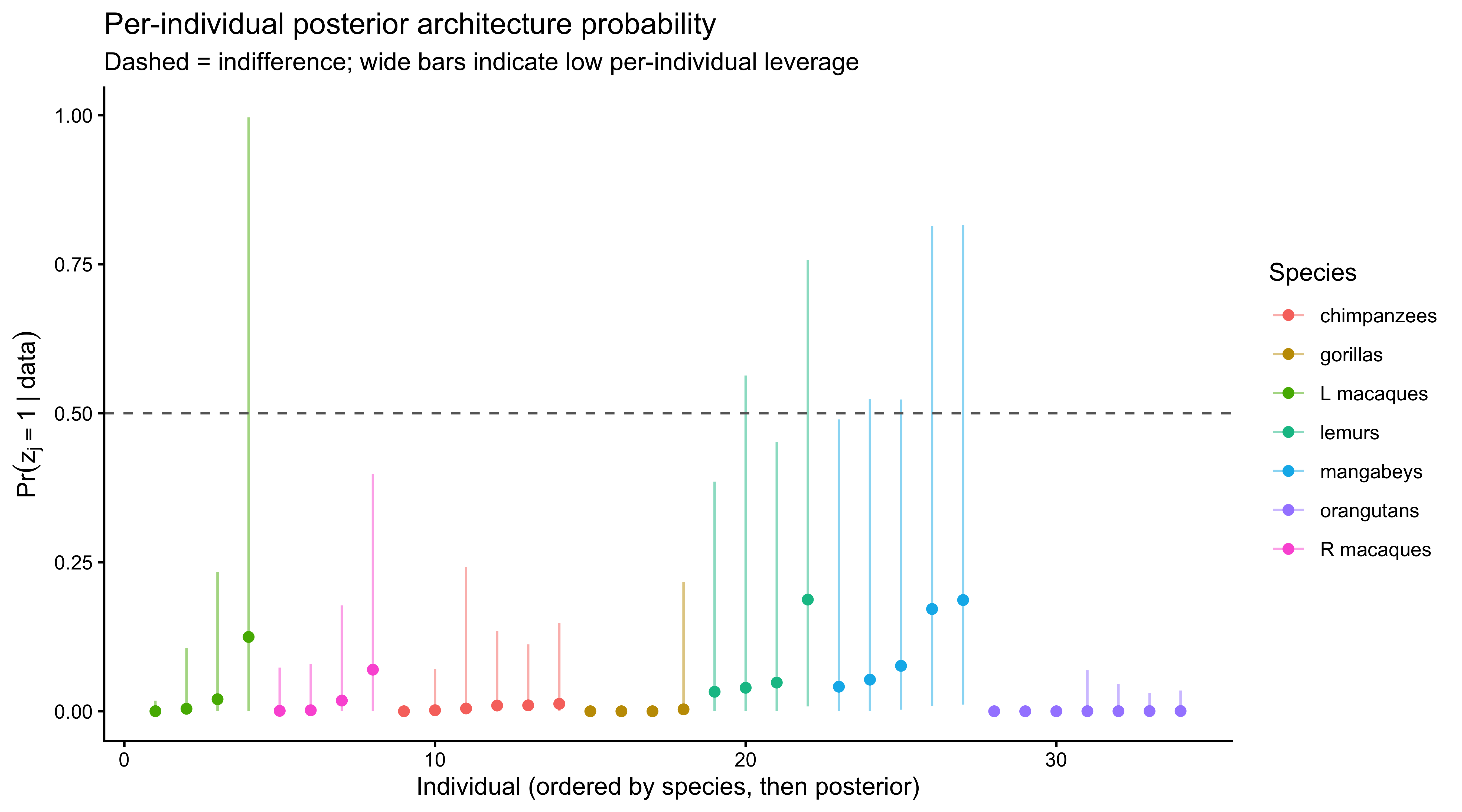
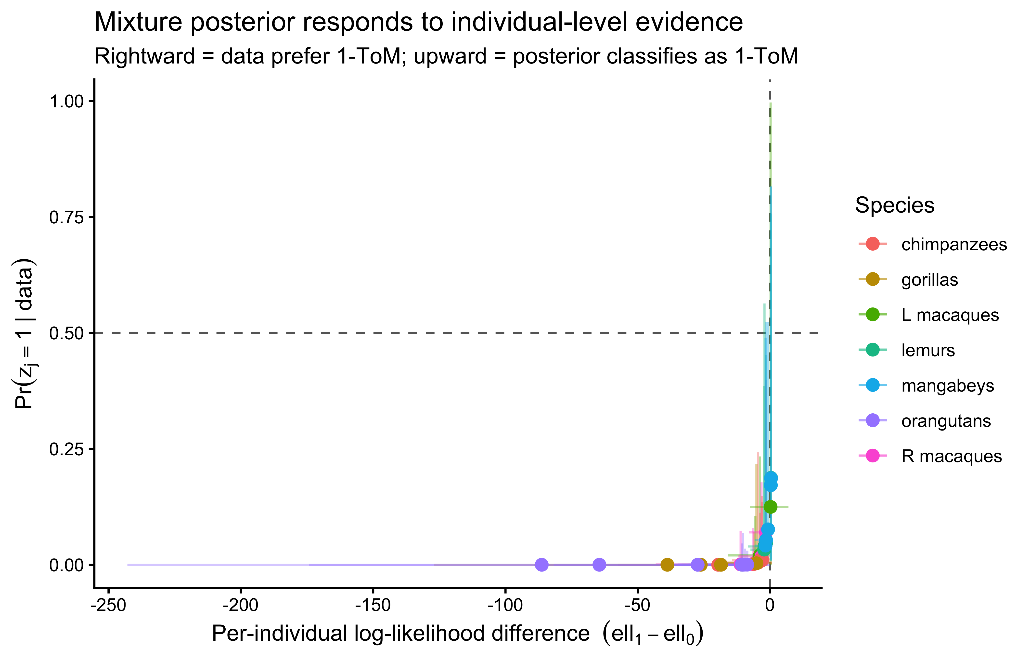
### Per-individual architecture posteriors
The mixture also delivers per-individual posterior probabilities
$\Pr(z_j = 1 \mid \text{data})$. Individuals whose data pull their
probability away from the species prior are those whose choice
sequences decisively fit one architecture over the other; those
whose posteriors return to the species prior $\pi_{s(j)}$ are
predictively indistinguishable under the two models, consistent with
the Occam's-razor evidence that matching pennies has limited
leverage at the single-individual scale.
```{r ch09_post_pi_ind, fig.width=9, fig.height=5, fig.cap="Per-individual posterior probability of being a 1-ToM agent, colored by species. Individuals close to 0 or 1 are cleanly classified by their data; those clustered near their species π_s reflect the limited per-individual leverage of matching pennies."}
post_pi_draws <- fit_mix$draws("post_pi_j", format = "df") |>
  as_tibble() |>
  dplyr::select(starts_with("post_pi_j")) |>
  pivot_longer(everything(), names_to = "param", values_to = "value") |>
  mutate(agent_id = as.integer(str_extract(param, "\\d+")))

post_pi_ind <- post_pi_draws |>
  group_by(agent_id) |>
  summarize(med = median(value),
            lo  = quantile(value, 0.05),
            hi  = quantile(value, 0.95),
            .groups = "drop") |>
  left_join(sd_int$agent_lookup, by = "agent_id") |>
  arrange(species, med) |>
  mutate(agent_id_ord = row_number())

ggplot(post_pi_ind, aes(x = agent_id_ord, y = med, color = species)) +
  geom_errorbar(aes(ymin = lo, ymax = hi), width = 0, alpha = 0.5) +
  geom_point(size = 1.8) +
  geom_hline(yintercept = 0.5, linetype = "dashed", color = "gray40") +
  labs(x = "Individual (ordered by species, then posterior)",
       y = expression(Pr(z[j]==1~"|"~data)),
       color = "Species",
       title = "Per-individual posterior architecture probability",
       subtitle = "Dashed = indifference; wide bars indicate low per-individual leverage")
```
### Sanity check against Occam's razor
Our Stan `generated quantities` block exposes two tightly-linked
per-individual quantities: `ll_diff_j` (the total log-likelihood
difference between the 1-ToM and 0-ToM arms at each posterior
draw's parameters) and `post_pi_j` (the Rao-Blackwellized posterior
probability that individual $j$ is a 1-ToM agent). If the mixture
is doing what it claims, individuals with larger `ll_diff_j` should
have higher `post_pi_j`, and the relationship should be a smooth
logistic curve rising from the species prior $\pi_{s(j)}$ at zero
evidence toward 1 at strong positive evidence. That curve is the
empirical operating characteristic of the mixture, and it is the
correct check to run — it confirms the mixture responds to
individual-level data, not only to the species-level covariates.
```{r ch09_mix_occam_check, fig.width=7, fig.height=4.5, fig.cap="Per-individual posterior architecture probability (y) vs. per-individual 1-ToM minus 0-ToM log-likelihood difference (x), both extracted from the mixture fit. Posterior-mean points, colored by species. A monotone rising curve confirms the mixture is actually responsive to the structural evidence in each individual's choices; flat clouds would indicate the posterior is driven entirely by the species-level prior."}
ll_diff_summary <- fit_mix$draws("ll_diff_j", format = "df") |>
  as_tibble() |>
  dplyr::select(starts_with("ll_diff_j")) |>
  pivot_longer(everything(), names_to = "param", values_to = "value") |>
  mutate(agent_id = as.integer(str_extract(param, "\\d+"))) |>
  group_by(agent_id) |>
  summarize(ll_diff_mean = mean(value),
            ll_diff_lo   = quantile(value, 0.05),
            ll_diff_hi   = quantile(value, 0.95),
            .groups = "drop")

mix_check <- post_pi_ind |>
  left_join(ll_diff_summary, by = "agent_id")

ggplot(mix_check, aes(x = ll_diff_mean, y = med, color = species)) +
  geom_hline(yintercept = 0.5, linetype = "dashed", color = "gray40") +
  geom_vline(xintercept = 0,   linetype = "dashed", color = "gray40") +
  geom_errorbar(aes(ymin = lo, ymax = hi), width = 0, alpha = 0.4) +
  geom_errorbarh(aes(xmin = ll_diff_lo, xmax = ll_diff_hi),
                 height = 0, alpha = 0.4) +
  geom_point(size = 2.5) +
  labs(x = expression("Per-individual log-likelihood difference "~(ell[1]-ell[0])),
       y = expression(Pr(z[j]==1~"|"~data)),
       color = "Species",
       title = "Mixture posterior responds to individual-level evidence",
       subtitle = "Rightward = data prefer 1-ToM; upward = posterior classifies as 1-ToM")
```
### How well does the mixture predict overall?
Mixture coefficients are only trustworthy to the extent that the
mixture model itself is predictively competitive. We compute PSIS-LOO
for the mixture and compare against the baseline hierarchical 0-ToM
(the non-mixture model fit earlier).
```{r ch09_mix_loo_compare}
loo_mix   <- fit_mix$loo()
loo_base  <- fit_hier$loo()
loo_cmp   <- loo::loo_compare(list(mixture = loo_mix, baseline_0tom = loo_base))
knitr::kable(as.data.frame(loo_cmp), digits = 2,
             caption = "PSIS-LOO comparison: mixture of architectures vs hierarchical 0-ToM only.")
```
A positive elpd_diff for `mixture` (with |elpd_diff| > 2·se_diff)
would indicate the extra 1-ToM arm is earning its complexity on
this dataset. A small or negative elpd_diff indicates that across
the 39 primates, the data jointly do not strongly prefer the
mixture — the species-level $\pi_s$ estimates would then carry
interpretive weight only insofar as they are shaped by the
covariate regression, not by individual-level likelihood contrast.
This is the predictive-calibration side of the same identifiability
story Phase 6 laid out: matching pennies is a game with limited
leverage for distinguishing architectures.
## Secondary analysis: decisional determinism within a 0-ToM architecture
The main analysis is complete. As a subsidiary question we now ask
whether, *conditional on treating every primate as a 0-ToM agent*,
species-level decisional determinism (`log_beta`) tracks ECV or
group size. This is the regression the previous version of this
chapter promoted to the main estimand; we now position it
correctly, as a question about statistical execution rather than
about representational capacity.
```{r ch09_write_stan_hier_reg}
stan_tom0_reg <- "
data {
  int<lower=1> N;
  int<lower=1> J;
  int<lower=1> S;
  array[J] int<lower=1, upper=S> species_of;
  array[N] int<lower=1, upper=J> agent;
  array[N] int<lower=0, upper=1> choice;
  array[N] int<lower=0, upper=1> op_choice;
  array[J] int<lower=1> start;
  array[J] int<lower=1> stop;
  vector[S] ecv_z;        // standardized log ECV
  vector[S] group_z;      // standardized log group size
}
parameters {
  vector[S] mu_log_sigma;
  real<lower=0> tau_log_sigma;
  vector[J] z_log_sigma;
  // log_beta regression
  real alpha_logbeta;
  real b_ecv;
  real b_group;
  real<lower=0> tau_sp;        // species residual SD on log_beta
  vector[S] z_sp;
  real<lower=0> tau_log_beta;  // individual-within-species SD
  vector[J] z_log_beta;
  // bias
  vector[S] mu_bias;
  real<lower=0> tau_bias;
  vector[J] z_bias;
}
transformed parameters {
  vector[S] mu_log_beta = alpha_logbeta + b_ecv * ecv_z +
                          b_group * group_z + tau_sp * z_sp;
  vector[J] log_sigma = mu_log_sigma[species_of] + tau_log_sigma * z_log_sigma;
  vector[J] log_beta  = mu_log_beta[species_of]  + tau_log_beta  * z_log_beta;
  vector[J] bias      = mu_bias[species_of]      + tau_bias      * z_bias;
  vector[N] dV;
  for (j in 1:J) {
    real sigma_j = exp(log_sigma[j]);
    real mu_s    = 0.0;
    real Sig_s   = 1.0;
    for (k in start[j]:stop[j]) {
      real s_mu = inv_logit(mu_s);
      real p_op = inv_logit(mu_s / sqrt(1 + 0.36 * Sig_s));
      dV[k] = 2 * p_op - 1;
      Sig_s = 1.0 / (1.0 / (Sig_s + sigma_j) + s_mu * (1 - s_mu));
      mu_s  = mu_s + Sig_s * (op_choice[k] - s_mu);
    }
  }
}
model {
  mu_log_sigma ~ normal(-2, 1);
  tau_log_sigma ~ exponential(2);
  z_log_sigma ~ std_normal();
  alpha_logbeta ~ normal(-1, 1);
  b_ecv   ~ normal(0, 0.5);
  b_group ~ normal(0, 0.5);
  tau_sp        ~ exponential(2);
  z_sp          ~ std_normal();
  tau_log_beta  ~ exponential(1);
  z_log_beta    ~ std_normal();
  mu_bias ~ normal(0, 1);
  tau_bias ~ exponential(1);
  z_bias ~ std_normal();
  for (n in 1:N)
    choice[n] ~ bernoulli_logit(
      (dV[n] + bias[agent[n]]) / exp(log_beta[agent[n]])
    );
}
generated quantities {
  vector[N] log_lik;
  for (n in 1:N)
    log_lik[n] = bernoulli_logit_lpmf(
      choice[n] | (dV[n] + bias[agent[n]]) / exp(log_beta[agent[n]])
    );
}
"
writeLines(stan_tom0_reg, here::here("stan", "ch09_tom0_reg.stan"))
mod_reg <- cmdstan_model(here::here("stan", "ch09_tom0_reg.stan"))
```
```{r ch09_prep_reg_data}
# Reuse species_cov from the mixture section; build the data list for
# the log_beta regression
sd_reg <- c(
  sd_int[c("N","J","S","species_of","agent",
           "choice","op_choice","start","stop")],
  list(ecv_z = species_cov$ecv_z,
       group_z = species_cov$group_z)
)
```
```{r ch09_fit_reg}
reg_path <- here::here("simmodels", "ch09_tom0_reg_fit.rds")
if (regenerate_fits || !file.exists(reg_path)) {
  fit_reg <- mod_reg$sample(
    data = sd_reg,
    chains = 4, parallel_chains = 4,
    iter_warmup = 1000, iter_sampling = 1000,
    adapt_delta = 0.95, seed = 2028
  )
  fit_reg$save_object(reg_path)
} else {
  fit_reg <- readRDS(reg_path)
}
fit_reg$diagnostic_summary()
```
### Results (decisional determinism)
```{r ch09_coef_plot, fig.width=10, fig.height=4, fig.cap="Secondary analysis: posterior coefficients of a regression of the 0-ToM decision temperature log_beta on species-level standardized log ECV and log group size. This is NOT the main estimand (see the mixture regression above) — it asks the narrower question of whether species act more deterministically on their 0-ToM predictions with larger brains or larger social groups. Negative coefficient = lower log_beta (tighter softmax) with higher covariate."}
coef_draws <- fit_reg$draws(c("b_ecv","b_group","alpha_logbeta","tau_sp"),
                            format = "df") |>
  as_tibble()

p_coef <- coef_draws |>
  dplyr::select(b_ecv, b_group) |>
  pivot_longer(everything(), names_to = "coef", values_to = "value") |>
  ggplot(aes(x = value, fill = coef)) +
  geom_density(alpha = 0.6, color = NA) +
  geom_vline(xintercept = 0, linetype = "dashed", color = "gray30") +
  scale_fill_manual(values = c("b_ecv" = "steelblue", "b_group" = "firebrick3"),
                    labels = c("b_ecv" = "ECV (scaffolding)",
                               "b_group" = "Group size (Machiavellian)")) +
  labs(x = expression(beta[cov]~"(log-beta per SD of log covariate)"),
       y = "Posterior density",
       fill = "Hypothesis",
       title = "Which covariate drives species-level decisiveness?",
       subtitle = "Mass to the left of 0 = lower log_beta (more deterministic) with larger covariate")

# Compare implied mu_log_beta from regression vs. baseline hier fit
baseline_mu <- fit_hier$draws("mu_log_beta", format = "df") |>
  as_tibble() |>
  summarize(across(starts_with("mu_log_beta"), mean)) |>
  pivot_longer(everything(), names_to = "param", values_to = "baseline_mean") |>
  mutate(species_id = as.integer(str_extract(param, "\\d+"))) |>
  left_join(species_cov |> dplyr::select(species_id, species), by = "species_id")

reg_mu <- fit_reg$draws("mu_log_beta", format = "df") |>
  as_tibble() |>
  summarize(across(starts_with("mu_log_beta"), mean)) |>
  pivot_longer(everything(), names_to = "param", values_to = "reg_mean") |>
  mutate(species_id = as.integer(str_extract(param, "\\d+")))

compare_df <- baseline_mu |> left_join(reg_mu, by = "species_id")

p_compare <- ggplot(compare_df, aes(x = baseline_mean, y = reg_mean, label = species)) +
  geom_abline(slope = 1, intercept = 0, linetype = "dashed", color = "gray40") +
  geom_point(size = 3, color = "midnightblue") +
  ggrepel::geom_text_repel(size = 3) +
  labs(x = "Baseline species mean log_beta",
       y = "Regression-implied species mean log_beta",
       title = "Do ECV + group size explain species variation?",
       subtitle = "Close to diagonal = covariates capture the between-species signal")

p_coef + p_compare + plot_layout(widths = c(1, 1))
```
The coefficient posteriors are the scientific payoff. Reading them
requires keeping the direction straight: `log_beta` is an *inverse*
measure of decisiveness — smaller values mean tighter softmax, more
deterministic use of the expected-utility signal. A *negative*
regression coefficient therefore means that species with higher ECV
(or larger groups) act more deterministically on their 0-ToM
predictions.
Summary statistics:
```{r ch09_coef_summary}
coef_summary <- coef_draws |>
  dplyr::select(b_ecv, b_group) |>
  pivot_longer(everything(), names_to = "coef", values_to = "value") |>
  group_by(coef) |>
  summarize(
    mean   = mean(value),
    median = median(value),
    q05    = quantile(value, 0.05),
    q95    = quantile(value, 0.95),
    p_neg  = mean(value < 0),
    p_pos  = mean(value > 0),
    .groups = "drop"
  )
knitr::kable(coef_summary, digits = 3)
```
Interpretation rests on whether each coefficient's 90% credible
interval excludes zero, on the sign, and on which of the two carries
more credible mass. Note well: with only seven species and two
correlated-but-not-collinear covariates, statistical power at the
species level is modest — this is an inference about an evolutionary
landscape sampled at seven points, and our uncertainty should reflect
that. An honest report sounds like "the posterior of $b_{\text{ECV}}$
places X% of mass below zero, while $b_{\text{group}}$ places Y%
below zero", not "ECV is the winner".
The second plot checks that the regression is sensible at all: if
the regression-implied species means fall close to the diagonal
against the non-regression baseline, then the covariates are
capturing most of the between-species variance. A scatter of points
far off the diagonal would indicate that ECV and group size jointly
miss an important species-level dimension (perhaps neocortex ratio,
diet, or rearing — all present in the raw CSV).
## Cross-check: species-level stacking weights
The mixture model delivered species-level architecture
probabilities $\pi_s$ as *parameters*, with full posterior
propagation. As a methodological cross-check, we can compare those
against species-level PSIS stacking weights computed from two
separately-fit hierarchical models (a pure-0-ToM hier and a
pure-1-ToM hier). The two estimators are answering related but
formally distinct questions — $\pi_s$ is a prior mixing proportion
inside a joint generative model, while stacking weights are
frequentist-flavored pseudo-BMA weights for out-of-sample
predictive averaging — so exact agreement is not expected, but gross
divergence would be concerning.
```{r ch09_stacking_crosscheck, fig.width=6, fig.height=5, fig.cap="Cross-check: species-level stacking weight for 1-ToM (x-axis, LOO-based pseudo-BMA) vs. mixture model posterior median π_s (y-axis). The two estimators answer related but formally distinct questions; gross divergence from the diagonal would indicate the mixture's π_s is driven by prior regularization rather than data. Error bars are 90% CIs on π_s from the mixture."}
loo0 <- fit_hier$loo()
loo1 <- fit_hier_tom1$loo()
species_of_trial <- sd_int$species_lookup$species[
  sd_int$species_of[sd_int$agent]
]
species_stack <- split(seq_along(species_of_trial), species_of_trial) |>
  imap_dfr(function(idx, sp) {
    lpd <- cbind(loo0$pointwise[idx, "elpd_loo"],
                 loo1$pointwise[idx, "elpd_loo"])
    w   <- loo::stacking_weights(lpd)
    tibble(species = sp, w_tom0 = w[1], w_tom1 = w[2])
  })

stack_compare <- species_stack |>
  left_join(pi_s_summary |> dplyr::select(species, med, lo, hi),
            by = "species")

ggplot(stack_compare, aes(x = w_tom1, y = med, label = species)) +
  geom_abline(slope = 1, intercept = 0, linetype = "dashed", color = "gray40") +
  geom_errorbar(aes(ymin = lo, ymax = hi), width = 0, alpha = 0.5,
                color = "steelblue") +
  geom_point(size = 3, color = "midnightblue") +
  ggrepel::geom_text_repel(size = 3) +
  coord_cartesian(xlim = c(0, 1), ylim = c(0, 1)) +
  labs(x = "Stacking weight for 1-ToM (LOO-based)",
       y = expression(pi[s] ~ "(mixture posterior median)"),
       title = "Stacking weights vs mixture \u03c0_s: cross-check",
       subtitle = "Diagonal = perfect agreement; deviations indicate regularization vs data-driven differences")
```
The mixture model is the principled version — it propagates
uncertainty, shares information appropriately across species via
the regression, and puts the scientific estimand on the right
scale. The stacking cross-check exists to verify that the mixture's
$\pi_s$ is not an artifact of prior-pulled regularization.
## Limitations
A candid list, because this chapter has pushed the framework as far
as it can honestly go on this dataset:
- **Fixed-parameter 1-ToM.** Our 1-ToM implementation tracks the
first two moments of the agent's belief about the opponent's
belief about itself, conditional on point values
$(\sigma_{\text{op}}, \beta_{\text{op}})$. The agent does not
represent uncertainty over those opponent parameters. The
full-variational scheme of Devaine et al. (2014a) does, and would
require a specialized message-passing backend to sample
efficiently. What we have estimated is therefore a 1-ToM agent
whose internal opponent model is a *fixed* 0-ToM with known
parameters, not a Bayesian learner over opponent sophistication.
- **Structural unidentifiability in matching pennies.** Phase 4b
SBC confirmed what the Devaine et al. (2014a) variational analysis
anticipates: $(\log\sigma_{\text{op}}, \log\beta_{\text{op}})$ are
weakly identified by matching-pennies choice sequences. Once
$\Sigma^{\text{self}}$ reaches its fixed point, the predicted
opponent-choice trajectory depends on these parameters only
through a compressed near-one-dimensional ridge. No amount of
Bayesian machinery can manufacture likelihood contrast that the
design does not provide. A reversal paradigm or a richer payoff
matrix is the appropriate remedy.
- **Mixture identifiability is design-bounded.** The per-individual
posterior $\Pr(z_j = 1)$ is informed only to the extent that
0-ToM and 1-ToM make differentiable predictions for that
individual — a leverage quantity we measured directly in the
Occam's-razor panel. Individuals whose choice sequences are
predictively equivalent under the two architectures have posteriors
that return to $\pi_{s(j)}$. This is correct Bayesian behavior,
but it means our species-level $\pi_s$ posteriors inherit the
design's limited per-individual separability.
- **Single-step reactive models.** 0-ToM, 1-ToM, and influence
learning all plan only one step ahead. They cannot strategically
deceive, willingly cooperate for long-run gain, or explore at the
cost of immediate reward. Repeated Prisoner's Dilemma exposes
every one of them.
- **2×2 games only.** The framework generalizes to arbitrary payoff
matrices, but both the primate study and this chapter live inside
a single-choice, two-option game. Naturalistic social interactions
are orders of magnitude richer, and richer settings are exactly
where higher-$k$ ToM should make a larger difference (Devaine et
al., 2017, Discussion).
- **Seven species is a small N.** The covariate regressions are
honest but statistically modest — an inference about an
evolutionary landscape sampled at seven points. The phylogenetic
structure of primates also means the species residuals around the
regression line are not independent in the usual sense (Devaine et
al., 2017 comment on this); a fuller analysis would embed a
phylogenetic variance-covariance on $u_s$.
- **Cooperative framing.** Primates partially read the game as
cooperative because their opponent is also their feeder. All of
our models have been written for the competitive payoff matrix; a
switch to cooperative incentives would flip signs in the influence
and 1-ToM equations and should be fit as a separate model (not
treated as noise).
- **No true $k \ge 2$.** The model set stops at $k = 1$. Devaine et
al. (2017) report an evolutionary gap between great apes and
humans precisely at $k = 2$, which our implementation cannot
currently reach. Extending the recursive belief-update machinery
to maintain a posterior over opponent sophistication level — and
adding a third mixture component — is the natural capstone
project.
- **A better predictive score is not a better mechanistic
explanation.** Ch. 7's caveat applies with extra force here.
Posterior architecture probability $\Pr(z_j = 1)$ summarizes
predictive structure in the choice sequences, not direct evidence
of mentalizing in the neurocognitive sense.
## Conclusion
We have traveled from *noticing* that a competitive game with an
adaptive opponent breaks the passive-environment assumption of
earlier chapters, through three computational instantiations of
that observation (0-ToM, influence learning, fixed-parameter
1-ToM), through a complete validation battery (prior predictive,
parameter recovery, SBC for both models, prior sensitivity,
posterior predictive, and an Occam's-razor model comparison
study), to a joint hierarchical mixture model that places
representational-capacity probabilities on the left-hand side of
the covariate regression and answers the actual scientific
question directly. Nothing in this pipeline is new machinery —
every tool came from Ch. 5, Ch. 6, or Ch. 7. What changed is what
the model is *about*: the object of inference is no longer a
statistical regularity but a mind that is modeling a mind, and the
estimand is not how sharply that mind acts but whether it is
mentalizing at all. That shift is what makes the chapter worth
writing, and it is the same shift that makes $k$-ToM one of the
most promising formal definitions on offer for a concept —
*theory of mind* — that has for decades existed as a verbal
construct in search of a mechanism.
## References
Daunizeau, J. (2014). The Variational Bayesian Approach (VBA)
toolbox. *Source code and documentation*, https://mbb-team.github.io/VBA-toolbox/.
Devaine, M., Hollard, G., & Daunizeau, J. (2014a). The social
Bayesian brain: does mentalizing make a difference when we learn?
*PLOS Computational Biology*, 10(12), e1003992.
Devaine, M., Hollard, G., & Daunizeau, J. (2014b). Theory of mind:
did evolution fool us? *PLOS ONE*, 9(2), e87619.
Devaine, M., San-Galli, A., Trapanese, C., Bardino, G., Hano, C.,
Saint Jalme, M., Bouret, S., Masi, S., & Daunizeau, J. (2017).
Reading wild minds: A computational assay of theory of mind
sophistication across seven primate species. *PLOS Computational
Biology*, 13(11), e1005833.
Hampton, A. N., Bossaerts, P., & O'Doherty, J. P. (2008). Neural
correlates of mentalizing-related computations during strategic
interactions in humans. *PNAS*, 105(18), 6741–6746.
Quesque, F., & Rossetti, Y. (2020). What do theory-of-mind tasks
actually measure? *Perspectives on Psychological Science*, 15(2),
384–396.
Schaafsma, S. M., Pfaff, D. W., Spunt, R. P., & Adolphs, R. (2015).
Deconstructing and reconstructing theory of mind. *Trends in
Cognitive Sciences*, 19(2), 65–72.
Talts, S., Betancourt, M., Simpson, D., Vehtari, A., & Gelman, A.
(2018). Validating Bayesian inference algorithms with
Simulation-Based Calibration. *arXiv:1804.06788*.
Waade, P. T., Enevoldsen, K. C., Vermillet, A.-Q., Simonsen, A., &
Fusaroli, R. (2022). Introducing tomsup: Theory of mind simulations
using Python. *Behavior Research Methods*, 55, 2197–2231.
Yao, Y., Vehtari, A., Simpson, D., & Gelman, A. (2018). Using
stacking to average Bayesian predictive distributions. *Bayesian
Analysis*, 13(3), 917–1007.