---
title: "The Design–Model Loop: Experimental (Re)Design as Part of Inference"
format:
html:
code-fold: true
code-tools: true
---
# The Design–Model Loop {#sec-appF}
```{r appf_setup, include=FALSE}
knitr::opts_chunk$set(
echo = TRUE,
warning = FALSE,
message = FALSE,
fig.width = 8,
fig.height = 5,
fig.align = 'center',
out.width = "85%",
dpi = 300
)
pacman::p_load(
tidyverse,
posterior,
cmdstanr,
tidybayes,
patchwork,
bayesplot,
here
)
set.seed(2026)
```
Across the book, several chapters reach a point where a model fails not because
the model is wrong but because the *experiment* cannot tell its parameters
apart. Chapter 5 showed that the memory agent's `bias` and `beta` are
collinear when the opponent plays a constant strategy, and the fix was a
*reversal* opponent. Chapter 13 showed that a decay rate $\lambda$ is
unidentifiable when nothing varies the time between observations. Chapter 17's
GCM-vs-rule comparison hinges on whether the stimuli are diagnostic between
the two models at all.
These are not three different problems. They are three faces of the same
fact: **the experimental design is part of the likelihood**, and so
identifiability, recovery, and model comparison are all properties of the
design as much as of the model. This appendix makes that fact formal and
gives you a small toolkit for diagnosing and improving designs *before* you
recruit a participant.
::: {.callout-tip title="How this appendix connects to the six-phase battery"}
You already have most of the machinery. The Phase 2 prior predictive, Phase 4
prior-to-posterior update, and Phase 6 recovery/SBC checks are *design
diagnostics in disguise*: each of them depends on the design $\xi$ as much as
on the model. This appendix re-reads the battery as a design loop and adds
two new utilities (Fisher information and Expected Information Gain) for the
cases where running full recoveries is too expensive.
:::
---
## 1. The design is part of the likelihood
Everywhere in the book we have written the likelihood as $p(y \mid \theta)$.
That notation hides something important. The probability of the observed
choices depends on what the participant saw — the opponent's sequence, the
stimuli, the inter-stimulus intervals, the feedback contingencies, the
number of trials. Collect all of those into a vector $\xi$ and write
$$
p(y \mid \theta, \xi).
$$
The parameter $\theta$ lives in the participant. The design $\xi$ lives in
the experimenter. The data $y$ are generated by their interaction.
Once $\xi$ is named, three things follow.
**First, the prior predictive is $\xi$-dependent.**
$$
p(y \mid \xi) = \int p(y \mid \theta, \xi)\, p(\theta)\, d\theta.
$$
"Does my model produce plausible behaviour?" is not a question about the
model alone; it is a question about the model *under a specific design*.
Same model, different design, different prior predictive.
**Second, identifiability is $\xi$-dependent.** A parameter that is
hopelessly confounded under one design can be sharply identified under
another. Bias and beta in Chapter 5 are the canonical example: the model
specification does not change between the failing and the working analysis;
only the opponent does.
**Third, the workflow is a loop, not a line.** Instead of
$$
\text{model} \to \text{fit} \to \text{publish or despair},
$$
we run
1. Propose a model $M$ and an initial design $\xi$.
2. Check the prior predictive $p(y \mid \xi)$. Is the spread of simulated
behaviour what the theory says it should be?
3. Score the design (recovery, contraction, EIG — see §2).
4. If the score is poor, revise $\xi$ (or, occasionally, $M$).
5. Pre-register, then run.
The "failed" parameter recovery in Chapter 5 is, in this view, the workflow
succeeding: it told us our design was weak *before* we used it on humans.
::: {.callout-note title="Power analysis is a special case"}
Classical power analysis asks: under a point alternative $\theta_1$ and a
fixed test, what design has $\geq 80\%$ chance of rejecting $\theta_0$?
That is a Bayesian Optimal Design problem with a degenerate prior (a point
mass) and a binary utility (reject vs. not). Everything we discuss below
generalizes power analysis to richer priors, continuous utilities, and
non-null model comparison.
:::
---
## 2. Design utility from cheap to expensive
There is no single "design utility" function — there is a ladder of them,
trading off cost against rigour. Pick the cheapest one that exposes your
failure mode.
### 2.1 Parameter recovery sweep (the cheapest)
Simulate datasets under several candidate designs $\{\xi_k\}$, fit the model
to each, and look at the recovery scatter. If `bias` and `beta` collapse onto
a ridge under $\xi_{\text{const}}$ and separate under $\xi_{\text{reversal}}$,
you have your answer in a single plot. This is what Chapter 5 actually does.
It costs you one Stan fit per design × ground truth.
### 2.2 Posterior contraction (an empirical EIG estimate)
For one or more representative $\theta^{*}$, contraction is
$$
C(\xi, \theta^{*}) = 1 - \frac{\mathrm{Var}\big(\theta \mid y, \xi\big)}{\mathrm{Var}\big(\theta\big)},
$$
with $y$ drawn from $p(y \mid \theta^{*}, \xi)$. Averaged over $\theta^{*}$
sampled from the prior, this is an empirical estimate of how much the
design lets you learn. Same cost order as recovery, but it gives you a
scalar utility per design — useful when comparing more than a handful.
### 2.3 Fisher Information (no fits required)
The Fisher Information Matrix at $\theta$ is
$$
\mathcal{I}(\theta; \xi) = -\mathbb{E}_{y \mid \theta, \xi}
\!\left[\nabla^{2}_{\theta} \log p(y \mid \theta, \xi)\right].
$$
If $\mathcal{I}(\theta; \xi)$ is (near-)singular at plausible $\theta$,
the design cannot locally distinguish parameter directions — this is what
"bias and beta are collinear" *means* mechanically. FIM is cheap (no
sampling), frequentist (no prior), and local (only valid near the $\theta$
you evaluate it at). Use it as a fast collinearity sniff test.
### 2.4 Expected Information Gain (the gold standard)
The Bayesian utility of a design $\xi$ is the expected KL divergence from
prior to posterior:
$$
\mathrm{EIG}(\xi) = \mathbb{E}_{p(y \mid \xi)}\!\Big[
\mathrm{KL}\big(p(\theta \mid y, \xi) \,\Vert\, p(\theta)\big)
\Big].
$$
EIG is prior-dependent (unlike FIM) and global (unlike FIM). It is also
expensive: the outer expectation is over $p(y \mid \xi)$, which itself is
a marginal over $\theta$. Naively, computing $\mathrm{EIG}(\xi)$ for one
design needs nested Monte Carlo — simulate datasets, fit each, average the
contractions. For a handful of candidate designs this is feasible; for a
search over a continuous space it is not, which is why §8 introduces
amortization.
The four utilities form a ladder. In practice we run recovery for the
final two or three candidates, contraction or FIM to pre-screen, and EIG
only when the design space is large enough to need a real optimization.
---
## 3. Case study: the reversal paradigm (Chapters 5–7) {#sec-appf-reversal}
In Chapter 5 the memory agent's choice probability is
$$
\Pr(y_t = 1 \mid \mathrm{bias}, \beta, h_{1:t-1}) =
\mathrm{logit}^{-1}\!\big(\mathrm{bias} + \beta\, \mathrm{logit}(\bar{h}_{t-1})\big),
$$
where $\bar{h}_{t-1}$ is the running mean of the opponent's choices
(clipped away from 0 and 1 before the logit, for numerical stability).
Writing $x_t = \mathrm{logit}(\bar{h}_{t-1})$ makes the design pathology
transparent: when the opponent plays a constant rate, $x_t$ converges to
a single value and the linear predictor collapses to
$\mathrm{bias} + \beta\, x^{*}$. Only the *sum* is identified; the
individual terms are not.
### 3.1 Fisher information makes the failure mechanical
For a single Bernoulli trial with linear predictor $\eta_t = \mathrm{bias}
+ \beta\, x_t$, the per-trial Fisher information matrix has the form
$$
\mathcal{I}_{t} = \sigma'(\eta_t)\;
\begin{pmatrix} 1 & x_t \\ x_t & x_t^{2} \end{pmatrix},
$$
where $\sigma'(\eta) = \sigma(\eta)(1-\sigma(\eta))$. The total
information $\sum_t \mathcal{I}_t$ is singular whenever $x_t$ is constant
across $t$: the second row is then a scalar multiple of the first. That
is the design pathology of the constant opponent, written in one line.
A reversal opponent — $p_{\text{opp}} = 0.8$ for the first half,
$p_{\text{opp}} = 0.2$ for the second (the Chapter 5 design) — gives two well-separated values
of $x_t$ once the running mean has stabilised in each block. The matrix
becomes well-conditioned, and bias and beta become jointly identified.
The Fisher information computation below uses the *asymptotic* per-block
covariate value $x = \mathrm{logit}(p_{\text{opp}})$ — a reasonable
approximation once $\bar{h}_t$ has converged within each regime. (For an
exact calculation across all trials, replace `x` by the full sequence of
$\mathrm{logit}(\bar{h}_{t-1})$ values that the Ch. 5 simulator
produces.)
```{r appf_fim_demo}
fim_two_block <- function(p_left, p_right, n_per_block,
                          bias = 0, beta = 1) {
  x_left  <- qlogis(pmin(pmax(p_left,  0.01), 0.99))
  x_right <- qlogis(pmin(pmax(p_right, 0.01), 0.99))
  x       <- c(rep(x_left, n_per_block), rep(x_right, n_per_block))
  eta     <- bias + beta * x
  w       <- plogis(eta) * (1 - plogis(eta))
  matrix(c(sum(w),     sum(w * x),
           sum(w * x), sum(w * x^2)), 2, 2)
}

designs <- tibble(
  label   = c("constant (p=0.5)", "weak split (0.6/0.4)",
              "reversal (0.8/0.2)"),
  p_left  = c(0.5, 0.6, 0.8),
  p_right = c(0.5, 0.4, 0.2)
) |>
  mutate(
    FIM       = map2(p_left, p_right, fim_two_block, n_per_block = 120),
    det_FIM   = map_dbl(FIM, det),
    cond_FIM  = map_dbl(FIM, ~ kappa(.x))
  )

designs |> select(label, det_FIM, cond_FIM)
```
A vanishing determinant and an exploding condition number are the FIM's
way of saying "this design cannot tell your parameters apart". You did not
need to fit a single model to see this.
### 3.2 The log-likelihood surface confirms the FIM diagnosis
The fastest empirical check on a design problem of this kind is to plot
the log-likelihood surface over $(\mathrm{bias}, \beta)$ for data
simulated under each design. A ridge means non-identification; a
contained blob means joint identification. No Stan fit needed — and no
calibration question to worry about, because we are visualising the
likelihood itself.
We use the exact Ch. 5 simulator (running-rate memory, clipped, logit
link on both `memory_input` and `theta`).
```{r appf_ch5_simulator}
# Verbatim from Chapter 5 (sec-model-quality-memory).
simulate_memory <- function(bias, beta, opponent_choices) {
  n_trials      <- length(opponent_choices)
  opp_rate      <- cumsum(opponent_choices) / seq_along(opponent_choices)
  memory_input  <- dplyr::lag(opp_rate, default = 0.5)
  memory_input  <- pmin(pmax(memory_input, 0.01), 0.99)
  theta_probs   <- plogis(bias + beta * qlogis(memory_input))
  self_choices  <- rbinom(n_trials, 1, theta_probs)
  tibble(trial = 1:n_trials,
         other_choice = opponent_choices,
         memory_state = memory_input,
         y = self_choices)
}

# Two designs, same ground truth. Matches Chapter 5's reversal design:
# N = 240 (120 trials per phase), opponent flips 0.8 -> 0.2 at trial 121.
set.seed(2026)
n_per_block   <- 120
opp_const     <- rbinom(2 * n_per_block, 1, 0.5)
opp_reversal  <- c(rbinom(n_per_block, 1, 0.8),
                   rbinom(n_per_block, 1, 0.2))

bias_true <- 0.0
beta_true <- 0.9

dat_const    <- simulate_memory(bias_true, beta_true, opp_const)
dat_reversal <- simulate_memory(bias_true, beta_true, opp_reversal)
```
```{r appf_loglik_surface, fig.width=9, fig.height=4.2}
loglik_surface <- function(dat, bias_grid, beta_grid) {
  x   <- qlogis(dat$memory_state)
  y   <- dat$y
  expand_grid(bias = bias_grid, beta = beta_grid) |>
    rowwise() |>
    mutate(
      ll = sum(dbinom(y, 1, plogis(bias + beta * x), log = TRUE))
    ) |>
    ungroup()
}

bias_grid <- seq(-2.0, 2.5, length.out = 80)
beta_grid <- seq(-1.0, 4.0, length.out = 80)

surf_const    <- loglik_surface(dat_const,    bias_grid, beta_grid) |>
  mutate(design = "constant opponent (p = 0.5)")
surf_reversal <- loglik_surface(dat_reversal, bias_grid, beta_grid) |>
  mutate(design = "reversal opponent (0.8 -> 0.2)")

# Centre each surface on its own maximum for visual comparability.
surf_all <- bind_rows(surf_const, surf_reversal) |>
  group_by(design) |>
  mutate(rel_ll = ll - max(ll)) |>
  ungroup()

ggplot(surf_all, aes(bias, beta, z = rel_ll)) +
  geom_contour_filled(breaks = c(-Inf, -50, -20, -10, -5, -2, -1, 0)) +
  geom_point(data = tibble(bias = bias_true, beta = beta_true),
             aes(x = bias, y = beta), inherit.aes = FALSE,
             colour = "white", size = 2.4) +
  facet_wrap(~ design) +
  scale_fill_viridis_d(option = "magma", direction = -1, name = "rel log-lik") +
  labs(title = "Log-likelihood under a constant vs. reversal opponent",
       subtitle = "Same model, same true parameters (white dot). Only the design differs.",
       x = "bias", y = "beta") +
  theme_minimal()
```
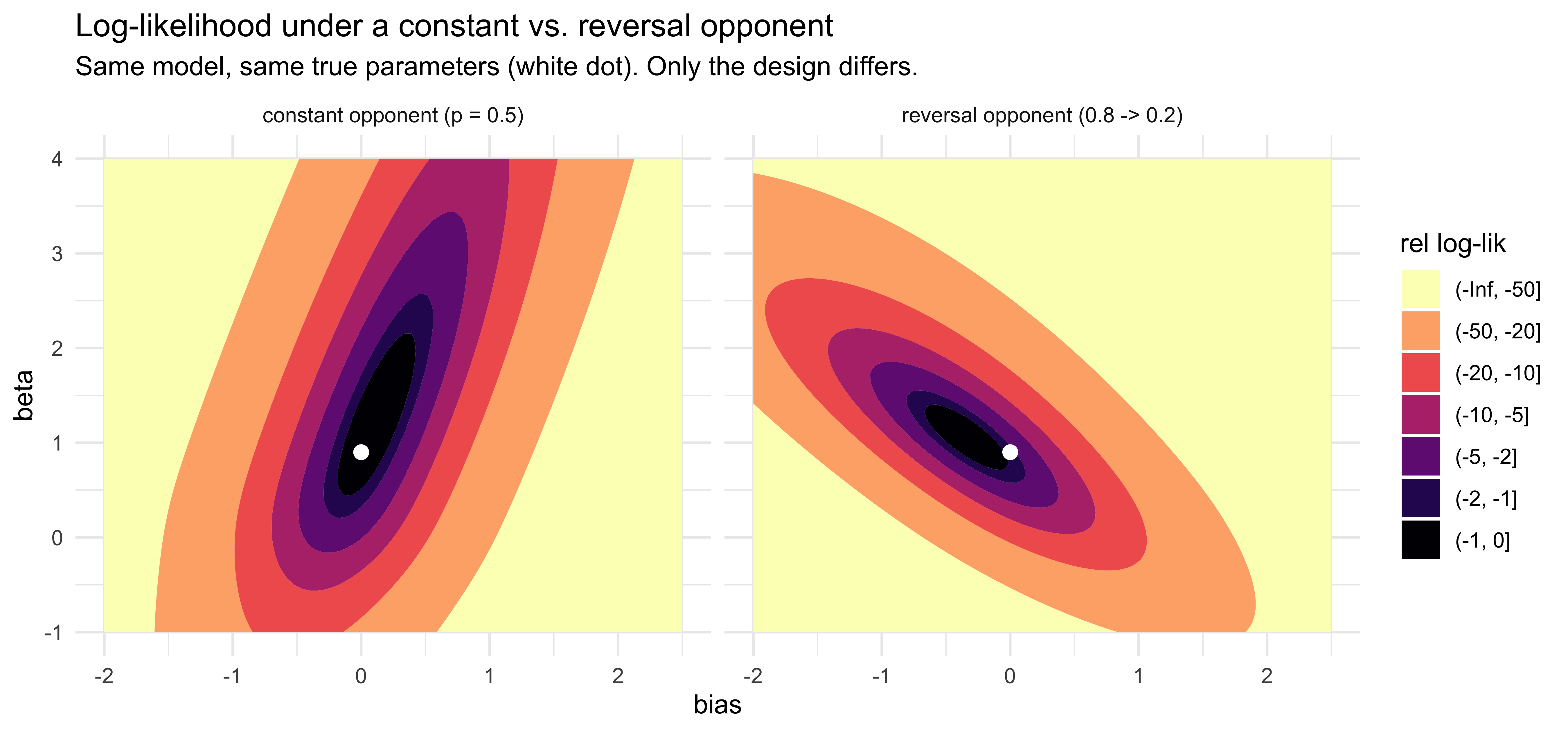
The two panels look very different even though the model and the true
parameters are identical. Under the constant opponent (left), the
cumulative running rate sits near $0.5$ throughout, so
$x = \operatorname{logit}(\text{memory}) \approx 0$ and the likelihood
depends on $\beta$ almost not at all: $\beta$ is essentially
unidentified, and the basin stretches vertically along the $\beta$ axis
while pinning $\mathrm{bias}$ near zero. Under the reversal opponent
(right), the running rate sweeps up toward $0.8$ in phase 1 and decays
back toward $0.5$ in phase 2, so $x$ now varies substantially and $\beta$
becomes identifiable. The basin is contained — bounded in both
directions — but still tilted, because the Chapter 5 memory is a
*cumulative* running rate and so $x$ is one-sided (mostly positive),
which leaves a residual $\mathrm{bias}$–$\beta$ correlation. The FIM
determinants in §3.1 predicted this ordering quantitatively *before* any
data were simulated; the surface here confirms it empirically. Running
HMC on these two datasets will reproduce the same picture — the
constant-opponent posterior will inherit a $\beta$-direction ridge; the
reversal posterior will produce a tilted but bounded cigar, which is
exactly the geometry Chapter 5 shows collapsing as $N$ grows.
### 3.3 Optimal reversal timing
The reversal does not have to land at the midpoint. Define $\tau$ as the
trial of the switch and consider $\mathrm{EIG}(\tau)$. Two intuitions:
- Too early: the first regime is under-sampled and bias is poorly pinned
down.
- Too late: the second regime barely contributes and the posterior is
effectively the constant-design posterior with an asymmetric correction.
You can compute $\mathrm{EIG}(\tau)$ analytically via the FIM determinant
for a Gaussian approximation, or empirically via the contraction sweep in
§2.2. For symmetric reversal magnitudes the optimum is near $\tau = N/2$;
for asymmetric ones (e.g.\ $p_{\text{opp}} = 0.5 \to 0.9$) the optimum
shifts towards the regime with less informative trials.
::: {.callout-tip title="What Chapter 5 was really doing"}
Chapter 5 narrates a model-fixing story ("we add a reversal"), but the
underlying move is a *design fix*. The model is unchanged. The same FIM
calculation generalizes: any time two parameters multiply the same
near-constant covariate, you have a design problem, and varying the
covariate is the fix.
:::
---
## 4. Case study: decay rates and environmental non-stationarity
A second family of models hits a structurally similar wall. Whenever a
parameter governs a *rate of change* — Ch. 13's forgetting rate
$\lambda$, Ch. 14's prototype process noise $q$, Ch. 15's rule-mutation
probability $\mu$ — that parameter is only identified if the design
*gives the agent something to forget about*, i.e., if the world is
non-stationary.
The mechanism is the same as in §3. In a static environment the decay
operates on a signal that does not change, so its effect on behaviour is
either zero (if the signal is already informative) or a constant
rescaling (if the signal contributes a smooth running average). Two
different $\lambda$'s produce indistinguishable behaviour. Vary the
environment — flip the categories halfway, drift the boundary, change
the reinforced rule — and the parameter governing forgetting becomes the
*single* parameter that controls how quickly the agent recovers. That
recovery curve is what identifies $\lambda$.
::: {.callout-note title="A note on 'temporal' decay"}
Some implementations of decay are indexed by elapsed *time* (so ISI
jitter is the design lever); the Ch. 13 model is indexed by *trial
number* (so the design lever is non-stationarity of the environment
across trials). Mathematically the situations are equivalent — both are
"vary the exposure" — but the practical knob is different. The Ch. 13
v2 chapter takes the trial-indexed route and tests three scenarios:
*static*, *contingent shift*, and *drift*.
:::
### 4.1 A minimal demonstration
We do not need the full GCM-with-decay simulator from Ch. 13 to see the
identifiability pattern. A two-line decay agent — a running rate
estimator with exponential downweighting of past observations —
reproduces the same FIM-singular behaviour under a static environment
and recovers $\lambda$ under a contingent shift.
The agent maintains a decay-weighted running mean
$$
\hat{r}_t = \frac{\sum_{s < t} e^{-\lambda (t - s)} z_s}{\sum_{s < t} e^{-\lambda (t - s)}},
$$
where $z_s \in \{0, 1\}$ is the signal observed on trial $s$ (e.g.\ the
true category, or whether the previous trial's response was correct),
and responds with $\Pr(y_t = 1) = \mathrm{logit}^{-1}(\alpha + \beta\,
\hat{r}_t)$ for fixed $\alpha, \beta$.
```{r appf_decay_sim}
decay_agent <- function(lambda, signal, alpha = 0, beta = 3) {
  n        <- length(signal)
  r_hat    <- numeric(n)
  for (t in 2:n) {
    s        <- 1:(t - 1)
    w        <- exp(-lambda * (t - s))
    r_hat[t] <- sum(w * signal[s]) / sum(w)
  }
  probs  <- plogis(alpha + beta * (r_hat - 0.5))
  list(r_hat = r_hat, probs = probs,
       y = rbinom(n, 1, probs))
}

# Two environments, both 200 trials.
set.seed(2026)
n_trials  <- 200
sig_static  <- rbinom(n_trials, 1, 0.7)                 # stationary
sig_shift   <- c(rbinom(n_trials/2, 1, 0.7),            # contingent shift
                 rbinom(n_trials/2, 1, 0.3))

lambda_true <- 0.10
sim_static  <- decay_agent(lambda_true, sig_static)
sim_shift   <- decay_agent(lambda_true, sig_shift)
```
### 4.2 The log-likelihood profile in $\lambda$
To check identifiability we profile the log-likelihood in $\lambda$ for
the simulated data, with $\alpha, \beta$ fixed at their generating
values. Under a static environment the running-rate agent still leaves
some fingerprint of $\lambda$ in its trial-by-trial response variance,
so the profile is not literally flat — but it is broad and biased.
Under a contingent shift, $\lambda$ also controls how fast the agent
catches up to the new regime, which adds a strong second source of
information; the profile becomes sharper and centred near the truth.
```{r appf_decay_profile, fig.width=8, fig.height=3.6}
profile_lambda <- function(signal, y, lambda_grid,
                           alpha = 0, beta = 3) {
  map_dbl(lambda_grid, function(lam) {
    sim_r <- decay_agent(lam, signal, alpha, beta)$probs
    sum(dbinom(y, 1, sim_r, log = TRUE))
  })
}

lambda_grid <- exp(seq(log(0.005), log(2.0), length.out = 60))

prof_static <- tibble(
  lambda = lambda_grid,
  ll     = profile_lambda(sig_static, sim_static$y, lambda_grid),
  design = "static environment"
)
prof_shift  <- tibble(
  lambda = lambda_grid,
  ll     = profile_lambda(sig_shift,  sim_shift$y,  lambda_grid),
  design = "contingent shift at t = 100"
)

bind_rows(prof_static, prof_shift) |>
  group_by(design) |>
  mutate(rel_ll = ll - max(ll)) |>
  ungroup() |>
  ggplot(aes(lambda, rel_ll)) +
  geom_line() +
  geom_vline(xintercept = lambda_true, linetype = "dashed", colour = "red") +
  scale_x_log10() +
  facet_wrap(~ design) +
  labs(title = "Profile log-likelihood for the decay rate",
       subtitle = "Dashed red line: true lambda. Broader/biased profile = weaker identification.",
       x = "lambda (log scale)", y = "rel log-lik") +
  theme_minimal()
```
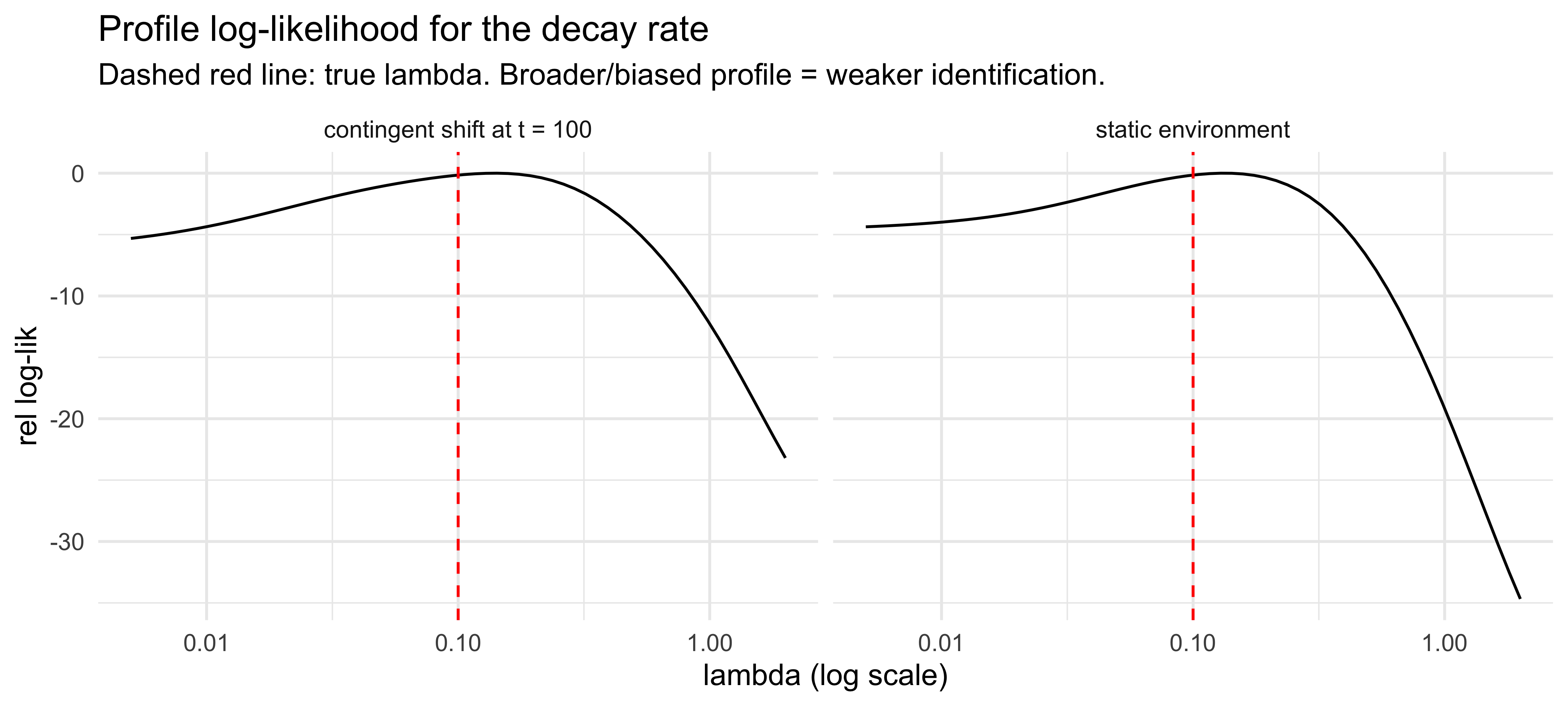
Both profiles peak near (slightly above) $\lambda_{\text{true}} = 0.1$,
but the *curvature* near the peak is what differs. The contingent-shift
profile (left) drops off sharply on both sides — the post-shift trials,
where high-$\lambda$ agents quickly track the new rate and low-$\lambda$
agents drag behind, supply strong information about $\lambda$ that is
robust to within-block noise. The static profile (right) is markedly
flatter on top: stationary data identify $\lambda$ only weakly, through
the variance structure of trial-by-trial fluctuations in $\hat{r}_t$,
so the maximum is poorly localised and a wide range of $\lambda$ values
fit the data nearly as well.
In the full Ch. 13 GCM-with-$\lambda$ the gap between the two designs
is even more dramatic. The GCM's response depends on the *ratio* of
summed similarities between categories, and under a static category
structure every additional exemplar reinforces its true category — so
the ratio is asymptotically insensitive to which exemplars are
downweighted by $\lambda$. The minimal model above keeps some residual
identification because it operates on a continuous rate; the categorical
version loses even that. Either way, the design lesson is the same: if
you want to identify a decay rate, the environment has to change.
### 4.3 Implications for the Ch. 13–15 designs
The same logic applies to all three categorization chapters:
- **Ch. 13 GCM with $\lambda$.** A *static* training schedule cannot
identify $\lambda$. The *contingent_shift* and *drift* scenarios in
the v2 chapter are not optional flourishes — they are what makes the
parameter recoverable at all.
- **Ch. 14 prototype Kalman with $q$.** Observation noise $r$ is
identified by within-category variance even in a static design.
Process noise $q$ is identified only by category drift. Under a
static schedule, $r$ and $q$ are individually weakly identified and
their *sum* is strongly identified — the same bias/beta pathology of
§3.
- **Ch. 15 rule particle filter with $\mu$.** $\mu$ governs the rate
at which the agent abandons a working rule. Without a covert rule
change in the design, the prior on $\mu$ never gets revised
meaningfully by the data.
The book's three-scenario standard (static / contingent_shift / drift)
is, in this framing, a three-design EIG sweep done by hand. Running each
model under each scenario and comparing parameter recovery is exactly
the contraction-based utility of §2.2.
---
## 5. The response format is part of the design: identifying precision parameters from binary choices {#sec-appf-response-format}
So far the design vector $\xi$ has collected stimulus-side choices — the
opponent's sequence, the reversal location, the candidate transfer
items. But $\xi$ also includes the *response format*: whether the
participant gives a binary choice, a confidence rating, a magnitude
estimate, a response time, or repeats the same trial many times. The
response format determines what likelihood we get to write down, and
some parameters in our cognitive models cannot be identified from a
binary likelihood no matter how cleverly the stimuli are arranged.
Chapter 11 already flags this in passing: the WBA precision parameter
$\kappa$ is "harder to pin down from binary outcomes" and "not helped
by more data — the problem is deeper". The same observation appears
elsewhere — the softmax inverse temperature $\phi$ in Chapter 4 and the
GCM specificity $c$ in Chapter 13 are all *scale* parameters that
modulate the *variance* of the choice distribution while leaving its
mean nearly unchanged. The pathology is the same one we have already
diagnosed twice in this appendix, just on a different axis of the
design space.
### 5.1 Why binary data starve precision parameters
For a Bernoulli observation $y \sim \text{Bern}(p(\theta, \xi))$, the
Fisher information about a parameter $\theta_k$ is
$$
\mathcal{I}_{kk} = \frac{(\partial p / \partial \theta_k)^2}{p(1-p)}.
$$
A parameter only earns information through its effect on the *mean* $p$.
If $\theta_k$ is a precision/concentration/inverse-temperature parameter
that — by construction — leaves $p$ approximately invariant (because the
mapping from the latent belief distribution to the choice probability
collapses across $\theta_k$), then $\partial p / \partial \theta_k
\approx 0$ and $\mathcal{I}_{kk} \approx 0$. This is exactly the WBA
$\kappa$ situation: rescaling $w_d$ and $w_s$ proportionally leaves the
Bayesian posterior mean $\hat{\theta}$ unchanged, so the binary choice
probability $\sigma(\text{logit}(\hat{\theta}))$ is also unchanged. The
information about $\kappa$ only leaks out through second-order effects
near the boundaries, where the posterior mean becomes sensitive to the
absolute weight scale.
The mechanical consequence: binary data identify $\kappa$ only weakly
and asymptotically; collecting *more* binary trials shrinks the
posterior on $\kappa$ very slowly, and no stimulus design can fully
undo this — the limitation is in the observation channel, not the
covariates.
```{r appf_kappa_binary_fim}
# Minimal WBA-style identification demo on a single conflict trial.
# Direct evidence "0.7 says blue", social evidence "0.7 says red";
# the Bayesian posterior is a Beta combination scaled by (w_d, w_s).
# Reparameterise as (rho, kappa).
posterior_mean <- function(rho, kappa, p_d = 0.7, p_s = 0.3) {
  w_d <- rho * kappa
  w_s <- (1 - rho) * kappa
  # Beta-style update with prior Beta(1,1) for simplicity:
  alpha <- 1 + w_d * p_d + w_s * p_s
  beta  <- 1 + w_d * (1 - p_d) + w_s * (1 - p_s)
  alpha / (alpha + beta)
}

# Sensitivity of choice probability to kappa, holding rho fixed:
rho_fix   <- 0.6
kappa_grid <- exp(seq(log(0.2), log(20), length.out = 60))
dp_dk <- numeric(length(kappa_grid))
for (i in seq_along(kappa_grid)) {
  eps <- 1e-3
  dp_dk[i] <- (posterior_mean(rho_fix, kappa_grid[i] + eps) -
               posterior_mean(rho_fix, kappa_grid[i] - eps)) / (2 * eps)
}

tibble(kappa = kappa_grid, dp_dkappa = dp_dk) |>
  ggplot(aes(kappa, abs(dp_dkappa))) +
  geom_line(linewidth = 0.8) +
  scale_x_log10() +
  labs(title = expression("Per-trial sensitivity of binary choice probability to " * kappa),
       subtitle = "rho = 0.6, conflict trial (p_d = 0.7, p_s = 0.3). Small values = weak Fisher information.",
       x = expression(kappa), y = expression(abs(partialdiff*p / partialdiff*kappa))) +
  theme_minimal()
```
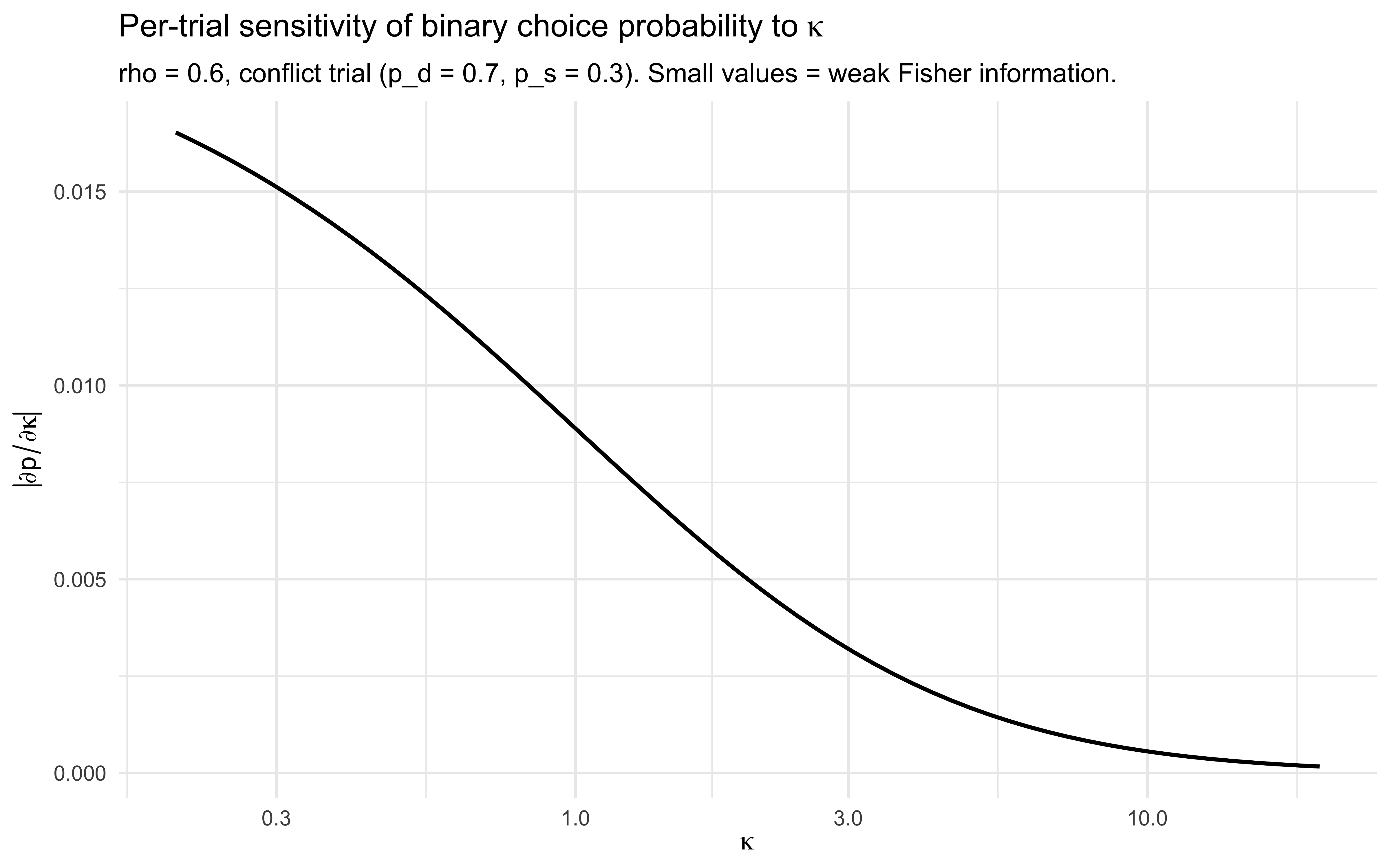
The slope $|\partial p / \partial \kappa|$ is small over the entire
plausible $\kappa$ range and decays toward zero as $\kappa$ grows.
Multiply by $1/(p(1-p))$ and sum across $N$ trials and you get the
per-trial Fisher information about $\kappa$ — a small number times $N$.
Doubling $N$ halves the posterior SD on $\kappa$, but you start from a
posterior SD large enough that no realistic experiment closes the gap.
### 5.2 What a richer response channel buys you
The fix is to widen the observation channel. Three response formats give
$\kappa$ a fighting chance, in increasing order of experimental effort:
**(a) Repeated identical trials.** If the same evidence configuration
$(p_d, p_s)$ is presented $R$ times, the empirical choice frequency on
that cell carries information about $p$, and *across-cell variation in
choice consistency* identifies $\kappa$. Mechanically: under
$y_{r} \sim \text{Bern}(p)$, the variance of the empirical mean is
$p(1-p)/R$, and the spread of cell-level consistencies across evidence
strengths is what $\kappa$ controls. This is the cheapest fix — same
binary response, just enforce within-cell replication.
**(b) Continuous confidence ratings.** Suppose the participant reports a
rating $r \in (0, 1)$ for "how confident are you that the next ball is
blue", and we model the rating as
$$
r \mid p, \kappa \sim \text{Beta}\!\big(\kappa\, p,\; \kappa\, (1-p)\big),
$$
where $p$ is the same Bayesian posterior mean as before. Now $\kappa$
appears directly in the rating likelihood as the concentration of the
Beta distribution: a high-$\kappa$ agent gives sharp, confident ratings,
a low-$\kappa$ agent gives noisy, near-uniform ratings. The Fisher
information about $\kappa$ from a single rating is bounded *below* by a
non-vanishing constant — independent of how far $p$ is from $0.5$.
**(c) Response times.** RT distributions carry independent information
about decision difficulty and noise. The drift-diffusion family
(@ratcliff_diffusion_2008) links a precision-like drift parameter to
both choice proportions *and* RT quantiles; fitting the joint
likelihood $p(y, \mathrm{RT} \mid \theta)$ identifies the precision
parameter from RT structure even when the binary choice is uninformative.
This is the most powerful response channel and the most demanding
modelling commitment — covering it properly is outside the scope of this
appendix, but the design principle is the same: extra response dimensions
unlock extra Fisher information.
### 5.3 Demonstration: $\kappa$ identification under three response formats
We simulate a small dataset from the WBA generative model and compute the
log-likelihood profile in $\kappa$ under three observation models on the
*same* trial sequence. The geometry is parallel to §3.2 (constant vs
reversal opponent) and §4.2 (static vs contingent-shift environment):
same model, same truth, different design — three very different
likelihoods.
```{r appf_kappa_profile, fig.width=9, fig.height=4}
# --- Simulate a small dataset from the WBA generative process ----------
set.seed(2026)
n_trials  <- 80
rho_true   <- 0.6
kappa_true <- 4
p_d <- runif(n_trials, 0.2, 0.8)
p_s <- runif(n_trials, 0.2, 0.8)

p_true <- mapply(posterior_mean, rho_true, kappa_true, p_d, p_s)

# Three response channels:
y_binary <- rbinom(n_trials, 1, p_true)
y_rating <- rbeta(n_trials,
                  shape1 = kappa_true * p_true,
                  shape2 = kappa_true * (1 - p_true))

# Replication: 8 evidence cells, 10 reps each.
cells <- expand_grid(p_d_cell = c(0.3, 0.5, 0.7, 0.8),
                     p_s_cell = c(0.3, 0.7))
reps  <- 10
p_cells <- mapply(posterior_mean, rho_true, kappa_true,
                  cells$p_d_cell, cells$p_s_cell)
y_rep <- rbinom(nrow(cells) * reps, 1,
                rep(p_cells, each = reps))

# --- Log-likelihood profiles in kappa, rho held at truth --------------
kappa_grid <- exp(seq(log(0.5), log(40), length.out = 60))

ll_binary <- map_dbl(kappa_grid, function(k) {
  p_k <- mapply(posterior_mean, rho_true, k, p_d, p_s)
  sum(dbinom(y_binary, 1, p_k, log = TRUE))
})

ll_rating <- map_dbl(kappa_grid, function(k) {
  p_k <- mapply(posterior_mean, rho_true, k, p_d, p_s)
  sum(dbeta(y_rating, k * p_k, k * (1 - p_k), log = TRUE))
})

ll_replicated <- map_dbl(kappa_grid, function(k) {
  p_k <- mapply(posterior_mean, rho_true, k,
                cells$p_d_cell, cells$p_s_cell)
  sum(dbinom(y_rep, 1, rep(p_k, each = reps), log = TRUE))
})

profile_df <- bind_rows(
  tibble(kappa = kappa_grid, ll = ll_binary,    channel = "1. binary only (N = 80)"),
  tibble(kappa = kappa_grid, ll = ll_replicated,channel = "2. replicated binary (8 cells x 10 reps)"),
  tibble(kappa = kappa_grid, ll = ll_rating,    channel = "3. binary + Beta rating (N = 80)")
) |>
  group_by(channel) |>
  mutate(rel_ll = ll - max(ll)) |>
  ungroup()

ggplot(profile_df, aes(kappa, rel_ll)) +
  geom_line(linewidth = 0.8) +
  geom_vline(xintercept = kappa_true, linetype = "dashed", colour = "red") +
  facet_wrap(~ channel, scales = "free_y") +
  scale_x_log10() +
  coord_cartesian(ylim = c(-30, 0)) +
  labs(title = expression("Profile log-likelihood for the precision parameter " * kappa),
       subtitle = "Dashed red line: true kappa. Sharper peak = better identification.",
       x = expression(kappa ~ " (log scale)"), y = "rel log-lik") +
  theme_minimal()
```
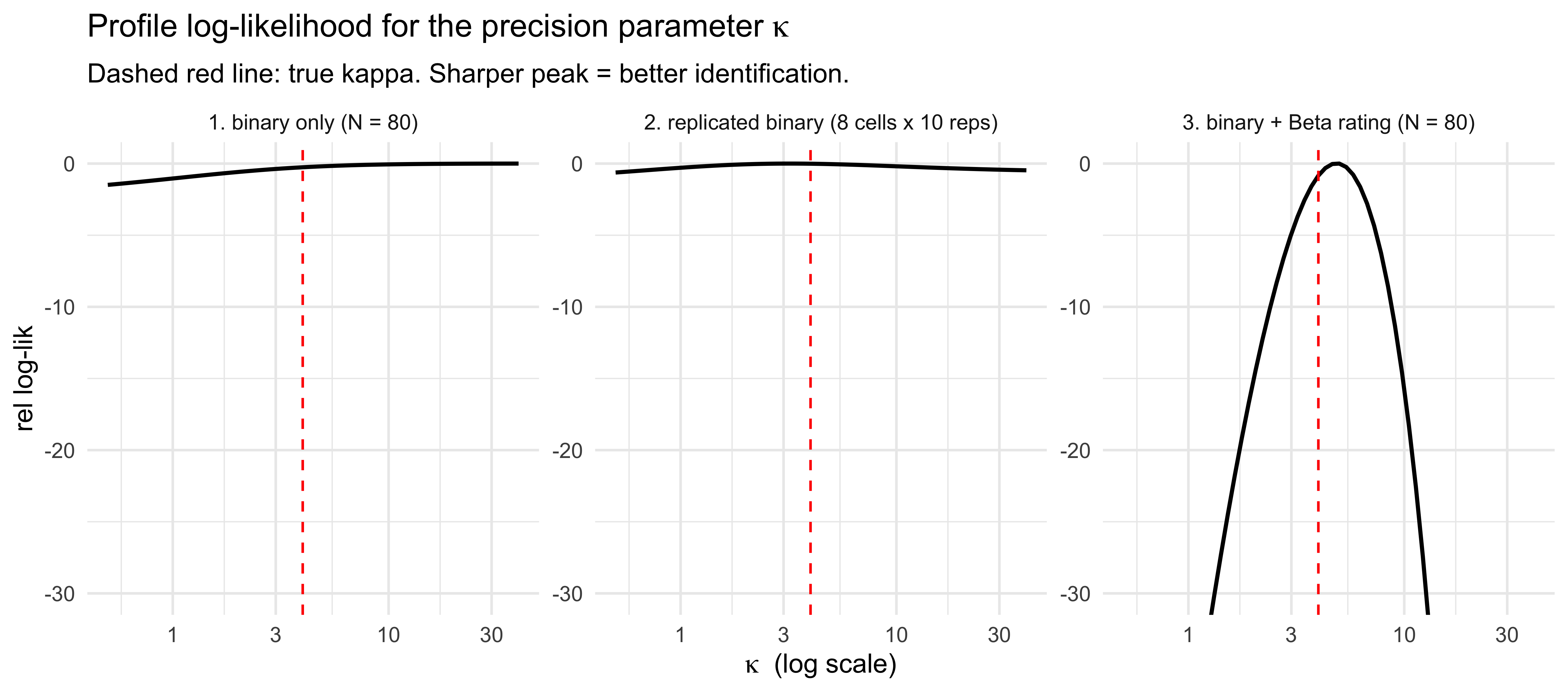
The binary-only profile (left) is essentially flat across the full
$\kappa$ range: with $N=80$ Bernoulli trials, every $\kappa$ in
$[0.5, 40]$ fits the data nearly as well as the truth. Replicating
binary trials within fixed evidence cells (centre) helps only modestly
at this sample size — within-cell choice variance does inform $\kappa$,
but slowly. The binary+rating profile (right) is dramatically sharper:
the Beta rating likelihood makes $\kappa$ a *mean-affecting* parameter
in the rating distribution, so it contributes non-vanishing Fisher
information on every trial and the profile collapses to a tight basin
around the truth. The qualitative ordering — *response channel matters
more than sample size* — is the practical headline.
### 5.4 Design rule and pointers to the chapters
Bring all of this together as a one-line rule:
> **If a parameter in your generative model scales the *variance* of the
> response distribution without moving its *mean*, binary outcomes will
> identify it only at the boundaries and asymptotically. To pin it down,
> either (a) replicate trials within fixed evidence cells, (b) collect a
> continuous response channel (confidence, magnitude estimate, slider
> probability) in which the parameter affects the mean of the response
> likelihood, or (c) collect response times and fit a joint
> choice-and-RT model.**
Read the binary-only comments in Chapter 11's WBA discussion, the
softmax-temperature observations in Chapter 4, and the GCM-specificity
identifiability discussion in Chapter 13 as three instances of this
same fact — and use this section as the place to plan around it before
the next experiment is run.
---
## 6. Model-discriminative design (Chapter 17)
Sometimes we don't care about $\theta$ — we care about which *model* the
participant is. The GCM-vs-rule comparison in Chapter 17 is the canonical
case.
Replace the parameter-estimation utility with the mutual information
between the model indicator $M$ and the data,
$$
I(M; y \mid \xi)
= \mathbb{E}_{p(M, y \mid \xi)}\!\left[
\log \frac{p(M \mid y, \xi)}{p(M)}
\right].
$$
A stimulus $\xi$ is *diagnostic* if it pushes models that look similar on
average behaviour far apart in their per-trial predictions. For
categorization specifically:
- A *prototype* model predicts near-identical responses for stimuli that
are equidistant from the prototype, regardless of where they sit.
- An *exemplar* model predicts substantially different responses for two
such stimuli if they are near vs. far from a specific stored exemplar.
So a model-discriminative stimulus set will deliberately include items
that are (a) equidistant from each category's prototype but (b) close to
exactly one stored exemplar of the training set. Prototype theory says
"same response"; exemplar theory says "very different responses". A
single trial of this kind contributes more to model comparison than
dozens of typical training-set items.
You can compute $I(M; y \mid \xi)$ by simulating from each candidate
model under the prior and counting how often the posterior over $M$
moves away from $0.5$. In practice this is cheap — you do not need to fit
either model; you only need to evaluate the predictive densities under
each.
---
## 7. Deep dive: discriminating GCM, prototype, and rule models {#sec-appf-cat}
Chapter 17 sets up a three-way comparison among an exemplar model (GCM, Ch
13), a prototype model (Kalman filter, Ch 14), and a rule-based model
(Bayesian particle filter, Ch 15). The diagnostics in that chapter (LOO,
PSIS, LFO) are *post hoc*: they tell you which model wins on data you
have already collected. The question this section asks is the *a priori*
counterpart: **what experiment maximizes your ability to tell these three
models apart in the first place?** And how is that different from running
three separate parameter-estimation optimizations, one per model?
### 7.1 The mimicry problem
Under a generic training-only design (a block of training items presented
i.i.d. from each category, no transfer set), the three models predict
near-identical accuracy trajectories. Each has free parameters that absorb
most of the qualitative differences:
- GCM ($c$, $w_1, w_2$): increasing sensitivity $c$ steepens the response
function; attention weights $w$ reshape the perceived distance.
- Prototype/Kalman ($r$, $q$): higher measurement noise $r$ flattens the
prototype's confidence; positive process noise $q$ keeps the prototype
drifting toward whichever category was seen most recently.
- Rule particle filter ($\mu$, $N$, $\varepsilon$): mutation probability
$\mu$ controls how readily the learner abandons a rule; particle count
$N$ controls the granularity of the rule posterior; $\varepsilon$ is a
lapse rate that flattens the response.
Any of the three can match a moderately steep training curve. Mimicry is
the rule, not the exception. If you ran posterior model comparison on
data from a generic training design, you would typically get diffuse
posterior weights over $M$ and an LOO difference within a few standard
errors of zero. Not because none of the models is right — because the
design did not put them in a position to disagree.
### 7.2 Optimizing within a single model: three different designs
Before tackling discriminability, note that even *intra-model* optima
differ across the three:
- **GCM-optimal.** To identify $c$ and the attention weights $w$, you need
stimuli that vary *along each feature dimension independently* and span
a wide similarity range. The attention weights are identified only when
the design forces a trade-off: stimuli where attending to dimension 1
predicts one response and attending to dimension 2 predicts another. A
feature-orthogonal stimulus set is the GCM-optimal core.
- **Prototype-optimal.** To identify $r$ (observation noise) and $q$
(process noise) separately, the design must vary the *category
variability* over time. Within-category variance pins down $r$; a
category drift or block-wise shift pins down $q$. A static category
structure makes $q$ unidentifiable in exactly the way Chapter 13's
decay parameter was.
- **Rule-optimal.** The rule particle filter is best identified when the
design escalates rule complexity across blocks (a 1-D rule, then a 2-D
conjunction, then a disjunction), as Kruschke (1993) does. $\mu$ is
identified by how rapidly behaviour adapts at each rule transition; $N$
by the residual variance after adaptation.
These three intra-model optima are not the same design. The GCM-optimal
design (feature-orthogonal, static categories) is *exactly* the design
under which the prototype model's $q$ is unidentifiable. The
rule-optimal design (escalating complexity across blocks) is one in which
the GCM's attention weights drift across blocks and you cannot pool
them. **"Optimize for all three models" is not a well-posed objective —
the three intra-model objectives conflict.**
### 7.3 The discriminative objective
The cross-model objective is structurally different. Rather than maximize
parameter EIG within any one model, we maximize the mutual information
between the model indicator $M$ and the data $y$ under the design $\xi$:
$$
I(M; y \mid \xi) = \sum_{M_k} p(M_k)\,
\mathbb{E}_{p(y \mid M_k, \xi)}\!\left[
\log \frac{p(y \mid M_k, \xi)}{\sum_j p(M_j)\, p(y \mid M_j, \xi)}
\right].
$$
The inner expectation is the average log-Bayes-factor that data $y$
contributes to model $M_k$ versus the marginal mixture. A stimulus is
diagnostic when this expectation is large in absolute value — equivalently,
when the three models *disagree on average* about $p(y \mid \xi)$.
This objective is qualitatively different from intra-model parameter
EIG. Parameter EIG rewards stimuli that resolve uncertainty *within* a
model's parameter space. Model-discriminative EIG rewards stimuli on
which the models, marginalized over their respective parameter spaces,
make different predictions. A stimulus can be highly informative for
estimating $c$ in the GCM while contributing nothing to discriminating
the GCM from the prototype model — and vice versa.
### 7.4 Where the three models disagree: design recipes
The diagnostic items are *transfer* items chosen so the three models'
marginal predictions diverge. Four families recur in the categorization
literature; all three can be expressed as design rules on the stimulus
space.
**(a) Prototype-only items.** Stimuli at the geometric centre of a
category but with no specific exemplar nearby (e.g., the centroid of
training items, if no training item sits exactly there).
- *Prototype model:* near-maximal confidence in the correct category
(the stimulus is exactly the central tendency).
- *GCM:* moderate confidence at best — summed similarity is bounded by
the *nearest* exemplars, none of which are close.
- *Rule model:* depends on the dominant rule; typically high confidence
*if* the rule names a feature value the centroid satisfies.
**(b) Exception items.** A training-set item that lies close to the
*opposite* category's prototype (the Medin & Schaffer 1978 5/4 structure
is the classic instance).
- *GCM:* correctly classifies (the exact exemplar is in memory).
- *Prototype model:* misclassifies or is at chance (the prototype is
averaged from training items that pull *away* from the exception).
- *Rule model:* depends on whether the active rule treats the
exception's features as decisive.
A single exception item, after sufficient training, contributes more to
GCM-vs-prototype discrimination than dozens of typical items.
**(c) Rule-vs-similarity items.** A stimulus that lies on the
*similarity-graded* side of a sharp rule boundary but with all other
features identical to a same-category training item.
- *Rule model:* sharp drop in $p(y = A)$ across the boundary,
independent of within-category similarity.
- *GCM and prototype models:* graded response that mostly ignores the
rule boundary (because their representations are similarity-based,
not threshold-based).
A pair of such items straddling the boundary yields a difference signal
that loads almost entirely on the rule-vs-similarity contrast.
**(d) Time-course probes.** Rule models predict piecewise-flat learning
curves with abrupt jumps at "insight" trials; similarity models predict
smooth, monotone curves. The diagnostic is *not* a stimulus — it is the
*trial structure*. Embedding a single block where the correct rule
changes silently (no instruction) produces a step response under rule
models and a slow drift under similarity models.
### 7.5 Building the diagnostic set computationally
You do not need analytic insight into which stimuli are diagnostic. The
calculation is cheap because no fitting is involved — only forward
simulation under each model's prior.
We work in the Kruschke (1993) 2D feature space used throughout Chs.
13–15. The training set is the eight Kruschke stimuli; the candidate
transfer set is a fine grid over the same space. We implement compact
versions of the three model architectures — the GCM simulator is the one
from Ch. 13 (lightly trimmed); the prototype model is a Gaussian
classifier over running per-category means (a stand-in for the Ch. 14
Kalman filter at its identifiability-relevant core); the rule model is a
1-feature threshold with lapse (a stand-in for the Ch. 15 particle
filter's marginal predictions over single-feature rules). The full
Chs. 13–15 simulators predict the *same qualitative* diagnostic
structure on these stimuli; the compact versions make the computation
finish in a few seconds.
```{r appf_cat_kruschke}
stimulus_info <- tibble(
  stimulus      = c(5, 3, 7, 1, 8, 2, 6, 4),
  height        = c(1, 1, 2, 2, 3, 3, 4, 4),
  position      = c(2, 3, 1, 4, 1, 4, 2, 3),
  category_true = c(0, 0, 1, 0, 1, 0, 1, 1)
)

training_obs <- as.matrix(stimulus_info[, c("height", "position")])
training_cat <- stimulus_info$category_true
```
```{r appf_cat_simulators}
# --- GCM (compact version of gcm_simulate from Ch. 13) ---------------
gcm_predict <- function(stim, training_obs, training_cat,
                        w, c, bias) {
  d    <- sqrt(colSums((t(training_obs) - stim)^2 * c(w, 1 - w)))
  sims <- exp(-c * d)
  m1   <- mean(sims[training_cat == 1])
  m0   <- mean(sims[training_cat == 0])
  num  <- bias * m1
  den  <- num + (1 - bias) * m0
  if (den < 1e-9) bias else num / den
}

# --- Gaussian prototype (compact stand-in for the Ch. 14 Kalman filter) ----
prototype_predict <- function(stim, training_obs, training_cat,
                              sigma, bias) {
  mu1 <- colMeans(training_obs[training_cat == 1, , drop = FALSE])
  mu0 <- colMeans(training_obs[training_cat == 0, , drop = FALSE])
  ll1 <- sum(dnorm(stim, mu1, sigma, log = TRUE))
  ll0 <- sum(dnorm(stim, mu0, sigma, log = TRUE))
  p1  <- bias * exp(ll1)
  p1 / (p1 + (1 - bias) * exp(ll0))
}

# --- Rule (compact stand-in for the Ch. 15 particle filter) ---------------
# A single-feature threshold rule with lapse rate eps.
rule_predict <- function(stim, dim, threshold, polarity, eps) {
  decision <- if (polarity == 1) stim[dim] > threshold else stim[dim] < threshold
  if (decision) 1 - eps else eps
}
```
```{r appf_cat_priors}
set.seed(2026)
n_draws <- 200

prior_gcm <- tibble(
  w    = runif(n_draws, 0.1, 0.9),
  c    = exp(rnorm(n_draws, mean = log(2), sd = 0.5)),
  bias = plogis(rnorm(n_draws, 0, 0.5))
)

prior_proto <- tibble(
  sigma = exp(rnorm(n_draws, mean = log(0.8), sd = 0.4)),
  bias  = plogis(rnorm(n_draws, 0, 0.5))
)

prior_rule <- tibble(
  dim       = sample(1:2, n_draws, replace = TRUE),
  threshold = runif(n_draws, 1.5, 3.5),
  polarity  = sample(c(-1, 1), n_draws, replace = TRUE),
  eps       = rbeta(n_draws, 2, 18)
)
```
```{r appf_cat_marginal}
# Candidate transfer locations: a 21x21 grid covering the Kruschke space
# plus a 1-cell margin.
candidates <- expand_grid(
  height   = seq(0.5, 4.5, length.out = 21),
  position = seq(0.5, 4.5, length.out = 21)
)

marginal_p <- function(stim, draws, model) {
  stim <- as.numeric(stim)
  preds <- switch(model,
    gcm   = mapply(function(w, c, b) gcm_predict(stim, training_obs, training_cat, w, c, b),
                   draws$w, draws$c, draws$bias),
    proto = mapply(function(s, b) prototype_predict(stim, training_obs, training_cat, s, b),
                   draws$sigma, draws$bias),
    rule  = mapply(function(d, th, po, ep) rule_predict(stim, d, th, po, ep),
                   draws$dim, draws$threshold, draws$polarity, draws$eps)
  )
  mean(preds)
}

pred_by_model <- candidates |>
  rowwise() |>
  mutate(
    p_gcm   = marginal_p(c(height, position), prior_gcm,   "gcm"),
    p_proto = marginal_p(c(height, position), prior_proto, "proto"),
    p_rule  = marginal_p(c(height, position), prior_rule,  "rule")
  ) |>
  ungroup() |>
  mutate(
    disagreement = sqrt(((p_gcm   - (p_gcm + p_proto + p_rule)/3)^2 +
                         (p_proto - (p_gcm + p_proto + p_rule)/3)^2 +
                         (p_rule  - (p_gcm + p_proto + p_rule)/3)^2) / 3)
  )
```
```{r appf_cat_plot, fig.width=8.5, fig.height=8.5}
plot_long <- pred_by_model |>
pivot_longer(c(p_gcm, p_proto, p_rule),
names_to = "model", values_to = "p_cat1") |>
mutate(model = recode(model,
p_gcm = "GCM",
p_proto = "Prototype",
p_rule = "Rule"))
p_models <- ggplot(plot_long, aes(position, height, fill = p_cat1)) +
geom_tile() +
geom_point(data = stimulus_info,
aes(position, height, colour = factor(category_true)),
inherit.aes = FALSE, size = 2) +
scale_fill_viridis_c(option = "viridis", limits = c(0, 1),
name = "P(y = 1)") +
scale_colour_manual(values = c("0" = "white", "1" = "black"),
name = "training cat") +
facet_wrap(~ model) +
coord_fixed() +
guides(colour = guide_legend(override.aes = list(size = 2))) +
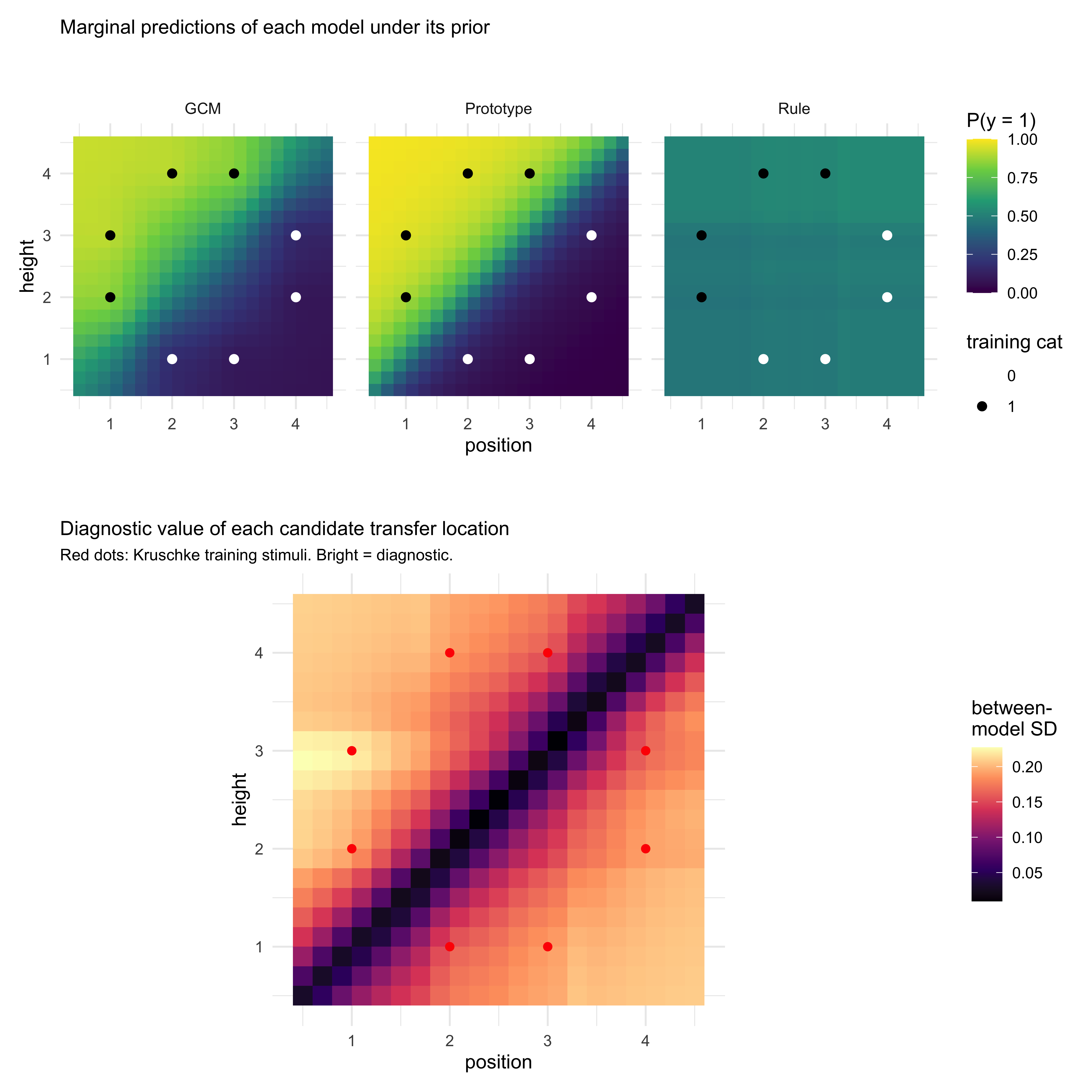
labs(title = "Marginal predictions of each model under its prior") +
theme_minimal(base_size = 11) +
theme(legend.position = "right",
plot.title = element_text(size = 11))
p_disagree <- ggplot(pred_by_model, aes(position, height, fill = disagreement)) +
geom_tile() +
geom_point(data = stimulus_info,
aes(position, height), inherit.aes = FALSE,
colour = "red", size = 1.8) +
scale_fill_viridis_c(option = "magma", name = "between-\nmodel SD") +
coord_fixed() +
labs(title = "Diagnostic value of each candidate transfer location",
subtitle = "Red dots: Kruschke training stimuli. Bright = diagnostic.") +
theme_minimal(base_size = 11) +
theme(legend.position = "right",
plot.title = element_text(size = 11),
plot.subtitle = element_text(size = 9))
p_models / p_disagree + plot_layout(heights = c(1, 1.2))
```
```{r appf_cat_diagnostic_set}
diagnostic_set <- pred_by_model |>
  slice_max(disagreement, n = 8) |>
  arrange(desc(disagreement))

diagnostic_set
```
Two things to read off the plot. First, the darkest band — the
*lowest*-disagreement region — runs along the centre diagonal of the
feature space, not through the training items. That is the implicit
*decision boundary*: at locations roughly equidistant from category-0
and category-1 exemplars, all three architectures predict close to
$0.5$, so they trivially agree on "I don't know". A transfer stimulus
placed there cannot discriminate the models. Second, the brightest
regions — the *most* diagnostic locations — sit *off* the diagonal and
*off* the training grid, at intermediate feature values where GCM,
prototype, and rule are forced to extrapolate in genuinely different
ways. This is exactly the kind of transfer geometry the
prototype-vs-exemplar literature has historically reached for by
intuition; here it is selected by computation.
For a tighter objective, replace the between-model SD with an empirical
estimate of $I(M; y \mid \xi)$: simulate binary responses under each
model and compute the average log-Bayes-factor that each candidate
stimulus contributes. The ranking is usually similar; the
mutual-information version is principled and runs in the same time
order.
::: {.callout-note title="Why compact stand-ins are honest here"}
The Ch. 14 Kalman prototype reduces, at the level of single-trial
marginal predictions, to a Gaussian classifier whose covariance depends
on the accumulated process and observation noise. The Ch. 15 particle
filter, marginalised over particles and rule complexities, predicts
near-thresholded responses on single features whose noise scales with
the mutation probability. Both compact versions reproduce the
*qualitative* prediction patterns that drive the between-model
disagreement structure. For an actual study, swap the compact
simulators for the Ch. 13–15 originals — the computation is the same,
only slower.
:::
### 7.6 The trade-off: model identifiability vs parameter identifiability
There is a price. A design tuned to maximize $I(M; y \mid \xi)$ tends to
*reduce* the within-model parameter EIG: diagnostic transfer items are
chosen precisely because they sit at locations where the models' average
predictions diverge, which often means locations where any single model's
prediction is relatively *insensitive* to its parameters (i.e., the
parameter gradients are small).
This is the categorization analogue of the classical estimation-vs-test
tension. You cannot maximize both unconstrained.
The practical compromise is a **two-phase design**:
1. *Training / estimation phase.* A standard training schedule (e.g., the
Kruschke 1993 stimulus set) that gives each model's parameters a fair
chance to be identified. This phase is roughly intra-model-optimal,
accepting that no single training schedule is jointly optimal for all
three (§7.2).
2. *Diagnostic phase.* A small set of transfer items chosen by the
computational recipe of §7.5, presented without feedback so the
parameter posteriors from Phase 1 are not perturbed.
Most published categorization studies use a version of this structure
implicitly. The contribution of the design-utility framing is to make
Phase 2 *computed* rather than *picked by hand* — and to make the
trade-off between phases explicit (how many trials to allocate to each is
a utility-allocation problem with the same EIG machinery on both sides).
### 7.7 Summary: three optima, one design
The categorization case makes the general lesson concrete:
- The GCM-optimal, prototype-optimal, and rule-optimal designs are
*different* designs. There is no design that is jointly optimal for
intra-model parameter estimation across all three.
- The model-discriminative design is *different again*. It optimizes a
different objective (the model indicator $M$, not the parameters
$\theta$), and rewards stimuli that the within-model objectives
consider uninformative.
- The realistic deliverable is a hybrid: a training phase that is
*defensible* (not optimal) under each model, followed by a diagnostic
transfer phase that is computed from the three models' prior
predictives. Chapter 17's three-way comparison is the analysis end of
this pipeline; this section is the design end.
---
## 8. Adaptive design optimization
Everything so far has been *static*: pick $\xi$ once, run the experiment,
analyze. The Bayesian generalization is *adaptive*: after trial $t$, pick
$\xi_{t+1}$ to maximize the EIG under the current posterior
$p(\theta \mid y_{1:t}, \xi_{1:t})$. This is the program of Adaptive
Design Optimization (Cavagnaro, Myung, Pitt, and colleagues).
There is a satisfying symmetry here with Chapter 11. In that chapter the
participant was a Bayesian agent updating beliefs about the world from
trial-by-trial feedback. In ADO, the *experimenter* is a Bayesian agent
updating beliefs about the participant from trial-by-trial responses,
and choosing the next stimulus to maximize expected learning. The two
loops are mathematically identical; only the roles are swapped.
For practical use in cognitive-science labs, ADO has three costs:
1. The next-stimulus EIG must be computed online, fast enough not to
stall the experiment. For small parameter spaces this is fine; for
the categorization models of Chapters 13–18 it is borderline.
2. The design is no longer pre-registered in the classical sense (the
exact stimulus sequence depends on the participant). Pre-registration
is still possible, but at the level of the *policy* that maps
posteriors to next stimuli rather than the sequence itself.
3. The analysis must condition on the adaptive policy or risk biased
inference — this is a feature of *any* sequential design, but ADO
makes it unavoidable.
When the experiment is long, participants are scarce, and the parameter
space is small (e.g.\ psychophysical thresholds), ADO is dramatic. For
the kind of multi-parameter learning models that this book centres on,
the gains are real but moderate, and the engineering cost is high.
---
## 9. Amortized design with NPE (bridge to @sec-appE)
The EIG of §2.4 is, naively, doubly intractable: an outer expectation
over $p(y \mid \xi)$ that itself marginalizes $\theta$, with inner
posteriors that have no closed form. Searching over a continuous design
space requires evaluating EIG at thousands of $\xi$ values. Nested Monte
Carlo makes this prohibitive.
This is exactly the setting where the amortized inference of
@sec-appE pays for itself. Once a Neural Posterior Estimator
$q_{\phi}(\theta \mid y)$ is trained on a wide range of $(\theta, \xi)$,
it gives you a *surrogate* posterior in microseconds. You can then:
- approximate $\mathrm{EIG}(\xi)$ by Monte Carlo over $\theta \sim p$
and $y \sim p(\cdot \mid \theta, \xi)$, using $q_{\phi}$ in place of
the true posterior;
- evaluate this for thousands of candidate $\xi$ in seconds;
- optimize $\xi$ by gradient ascent if $\xi$ is continuous (using the
same auto-diff that trained $q_{\phi}$).
The frontier here — Foster et al.'s DAD/iDAD line of work — trains a
*design network* jointly with the inference network, so that the next
stimulus is produced as a forward pass through a small neural net at
test time. This pushes ADO into regimes that classical methods cannot
reach. For the models in this book it is overkill; for the next
generation of large categorization studies it will not be.
::: {.callout-warning title="Frontier territory"}
The amortized-BOED literature is moving fast and the engineering is not
yet plug-and-play. The cost-benefit for student projects is poor today.
Use the static and recovery-based diagnostics of §2–§4 for the
experiments you are designing this term; treat §8 as a road sign for the
direction the field is heading.
:::
---
## 10. Practical constraints and the design–theory loop
A pure EIG-maximizer will hand you a design that maximizes information
per unit experimenter time and ignores every constraint that actually
binds your study: participants get tired, ISIs cannot be negative,
ethics boards do not approve 4-hour sessions, the lab MRI is booked, the
stimuli have to be counterbalanced across condition, and the response
modality has a floor on reaction time.
The right way to handle this is to encode constraints as a feasible set
$\Xi \subset \Xi_{\text{ideal}}$ and (optionally) attach a cost $c(\xi)$
to candidate designs, so that the utility you actually optimize is
$$
U(\xi) = \mathrm{EIG}(\xi) - \lambda\, c(\xi), \qquad \xi \in \Xi.
$$
Doing so makes the trade-offs explicit. "We added 20 minutes to the
session" becomes "we gained $\Delta\mathrm{EIG}$ at a cost
$\lambda\, \Delta c$, which is justified iff $\Delta\mathrm{EIG} >
\lambda\, \Delta c$."
A non-exhaustive checklist for real experiments:
- **Fatigue**: utility per trial decreases over a session. Implicit cost
on session length.
- **Dropout**: longer sessions lose participants non-randomly. Cost on
the data you do *not* get.
- **Carry-over**: information from earlier trials can change later
trials' likelihood (Chapter 5's memory agent is the within-task
version of this; between-block carry-over is the cross-block version).
- **Counterbalancing**: necessary for causal claims, often costs EIG.
- **Ethics**: hard constraints. Encode as $\xi \notin \Xi$.
- **Pilot data**: the prior $p(\theta)$ is rarely known a priori. Use a
pilot to set it, and recompute EIG; this turns design into an
iterative process across studies, not just within one.
### The loop, in full
Putting §1–§10 together, the workflow you should run before any new
experiment is:
1. Specify $M$ and a candidate $\xi$.
2. Prior predictive under $\xi$: does the behaviour look like the
theory?
3. FIM at plausible $\theta$: any collinear directions? If so, change
$\xi$.
4. Recovery + contraction at a handful of $\theta^{*}$: do the
parameters you care about contract?
5. If the design space is large or continuous, approximate EIG
(amortized if needed) and optimize within the feasible set $\Xi$.
6. SBC under the chosen $\xi$ to confirm calibration.
7. Pre-register; run.
The "failed" recoveries scattered through this book are not the
embarrassments they look like in isolation. They are the loop working.
The job of Bayesian workflow is to surface those failures *on simulated
data*, where the cost of failure is a Stan rerun rather than a lost
cohort. The design–model loop is what makes that possible.
---
::: {.callout-note title="Further reading"}
- Lindley (1956), *On a measure of the information provided by an
experiment*, **Ann. Math. Statist.** — the original definition of EIG.
- Chaloner & Verdinelli (1995), *Bayesian Experimental Design: A
Review*, **Statist. Sci.** — the canonical survey.
- Cavagnaro, Myung, Pitt & Kujala (2010), *Adaptive Design Optimization*,
**Neural Comput.** — ADO in cognitive science.
- Ryan, Drovandi, McGree & Pettitt (2016), *A Review of Modern
Computational Algorithms for Bayesian Optimal Design*,
**Internat. Statist. Rev.** — Monte Carlo machinery.
- Foster, Ivanova, Malik & Rainforth (2021), *Deep Adaptive Design*,
**ICML** — amortized BOED via neural networks.
- Rainforth, Foster, Ivanova & Smith (2024), *Modern Bayesian
Experimental Design*, **Statist. Sci.** — current state of the art.
:::