# Sequential Extensions of the Bayesian Agent {#sec-bayesian-sequential-extensions}
```{r ch11_setup, include=FALSE}
knitr::opts_chunk$set(
echo = TRUE,
warning = FALSE,
message = FALSE,
fig.width = 8,
fig.height = 5,
fig.align = 'center',
out.width = "80%",
dpi = 300
)
# Flag to control whether to regenerate simulations/fits
# Set to TRUE to rerun everything, FALSE to load saved results.
regenerate_simulations <- FALSE
# Create directories if they don't exist
for (d in c("stan", "simdata", "simmodels", "figures")) {
if (!dir.exists(d)) dir.create(d)
}
pacman::p_load(
tidyverse,
cmdstanr,
posterior,
bayesplot,
patchwork,
here
)
theme_set(theme_minimal())
```
Every Bayesian agent we built in Ch. 10 — SBA, WBA, PBA, and their
multilevel cousins — shares two strong assumptions. First, the agent is
*forced* to guess on every trial: there is no option to defer, ask for
more evidence, or decline. Second, the weights on direct and social
evidence are *static*: whatever trade-off an agent starts with, they
carry it through the entire experiment unchanged. Both assumptions are
reasonable first-pass idealisations, and both are almost certainly false
about real cognition.
This appendix sketches two extensions that relax each assumption in turn.
Section A introduces a **sample-or-guess agent** that decides at every
step whether to collect more evidence or commit to a choice. Section B
introduces an **adaptive-weight agent** whose weights drift across
trials in response to how well each source predicted recent feedback.
> **Scope note.** These two models are offered as *starting points for
> student projects*, not as fully validated contributions. We give the
> mathematical formalization, an R forward simulation, visualisations of
> the agents' behaviour, and a single-agent Stan model fit once for
> illustration. We deliberately omit parameter recovery, SBC, model
> comparison, and multilevel extensions — all of these are natural next
> steps and good exercises. Treat what follows as a skeleton to build on.
## Section A: Sample-or-Guess Agent
### Conceptual motivation
The agents in Ch. 10 are committed decision-makers: evidence arrives, they
integrate it, and they respond. In many real tasks — clinical diagnosis,
foraging, perceptual decision-making under time pressure — the agent
instead chooses *when to stop sampling*. A cautious agent keeps
observing marbles until confident; an impulsive one guesses after the
first draw. The trade-off is classical: more samples mean better
accuracy but higher cost (time, effort, missed opportunities). This
family of policies connects the Bayesian-cognition literature to
sequential-sampling models of reaction time (e.g., the drift-diffusion
model) and to metacognition, where confidence gates commitment.
The key conceptual move is that the observation model now has *two*
outputs per trial. On every step the agent emits a stop/continue
decision; when it finally stops, it emits a guess. The likelihood must
account for both — a point that is easy to miss when porting the Ch. 10
Stan templates.
### Mathematical formalization
Let trial $i$ consist of a sequence of evidence draws. The agent enters
the trial with a prior (we use Jeffreys: $\alpha_0 = \beta_0 = 0.5$) and
an optional social tip summarised as $(k_s, n_s)$. After observing
direct evidence up to step $t$ — $k_{d,t}$ blue out of $t$ direct draws
— the posterior over the jar's blue proportion $\theta$ is
$$\theta \mid \text{evidence}_t \sim \text{Beta}(\alpha_t,\, \beta_t),$$
with
$$\alpha_t = 0.5 + k_s + k_{d,t}, \qquad
\beta_t = 0.5 + (n_s - k_s) + (t - k_{d,t}).$$
Define the agent's **certainty** at step $t$ as
$$c_t \;=\; \left|\, \mathbb{E}[\theta \mid \text{evidence}_t] - 0.5 \,\right|
\;=\; \left|\, \frac{\alpha_t}{\alpha_t + \beta_t} - 0.5 \,\right|.$$
The agent's policy is governed by a single free parameter $\tau \in
(0, 0.5)$:
$$
\text{at step } t: \quad
\begin{cases}
\text{stop, guess } g_i = \mathbf{1}[\alpha_t > \beta_t] & \text{if } c_t \ge \tau, \\
\text{draw one more marble, increment } t & \text{otherwise.}
\end{cases}
$$
The data observed per trial are the stopping time $T_i$ and the final
guess $g_i$. The likelihood factorises as
$$p(T_i, g_i \mid \tau, \text{evidence}) \;=\;
\underbrace{\prod_{t=1}^{T_i - 1} \Pr(\text{continue at } t \mid \tau)}_{\text{didn't stop earlier}}
\;\cdot\;
\underbrace{\Pr(\text{stop at } T_i \mid \tau)}_{\text{stops now}}
\;\cdot\;
\underbrace{\Pr(g_i \mid \alpha_{T_i}, \beta_{T_i})}_{\text{final guess}}.$$
Two important caveats. **First**, after the agent stops, the would-be
marbles at steps $T_i + 1, T_i + 2, \ldots$ are *not* observed. Trials
are not i.i.d. sequences of a fixed length; the data are censored by the
agent's own decision. **Second**, the hard-threshold rule above is
non-differentiable in $\tau$, which breaks HMC. For inference we
therefore replace it with a soft version,
$$\Pr(\text{stop at } t \mid \tau) \;=\; \sigma\!\left(\frac{c_t - \tau}{\sigma_\tau}\right),$$
where $\sigma(\cdot)$ is the logistic function and $\sigma_\tau$ is a
small fixed slope (we use $\sigma_\tau = 0.02$). As $\sigma_\tau \to 0$
the soft rule recovers the hard one.
### R forward simulation
```{r ch11_threshold_agent_fn}
# Simulate one agent with a hard certainty threshold.
# Returns a tibble with one row per trial.
simulate_threshold_agent <- function(tau,
                                     n_trials,
                                     max_samples = 30,
                                     true_theta = 0.7,
                                     social_k = 1,
                                     social_n = 3,
                                     alpha0 = 0.5, beta0 = 0.5) {
  purrr::map_dfr(seq_len(n_trials), function(trial) {
    alpha_t <- alpha0 + social_k
    beta_t  <- beta0  + (social_n - social_k)
    stopped <- FALSE
    t <- 0
    while (!stopped && t < max_samples) {
      c_t <- abs(alpha_t / (alpha_t + beta_t) - 0.5)
      if (c_t >= tau && t >= 1) {
        stopped <- TRUE
      } else {
        t <- t + 1
        draw <- rbinom(1, 1, true_theta)  # 1 = blue, 0 = red
        alpha_t <- alpha_t + draw
        beta_t  <- beta_t + (1 - draw)
      }
    }
    guess <- as.integer(alpha_t > beta_t)
    tibble(
      trial   = trial,
      tau     = tau,
      T       = t,
      guess   = guess,
      correct = as.integer(guess == as.integer(true_theta > 0.5))
    )
  })
}

# Three agents with different thresholds
sim_threshold <- bind_rows(
  simulate_threshold_agent(tau = 0.10, n_trials = 200),
  simulate_threshold_agent(tau = 0.25, n_trials = 200),
  simulate_threshold_agent(tau = 0.40, n_trials = 200)
) |>
  mutate(tau_label = factor(paste0("tau = ", tau)))
```
### Visualisations
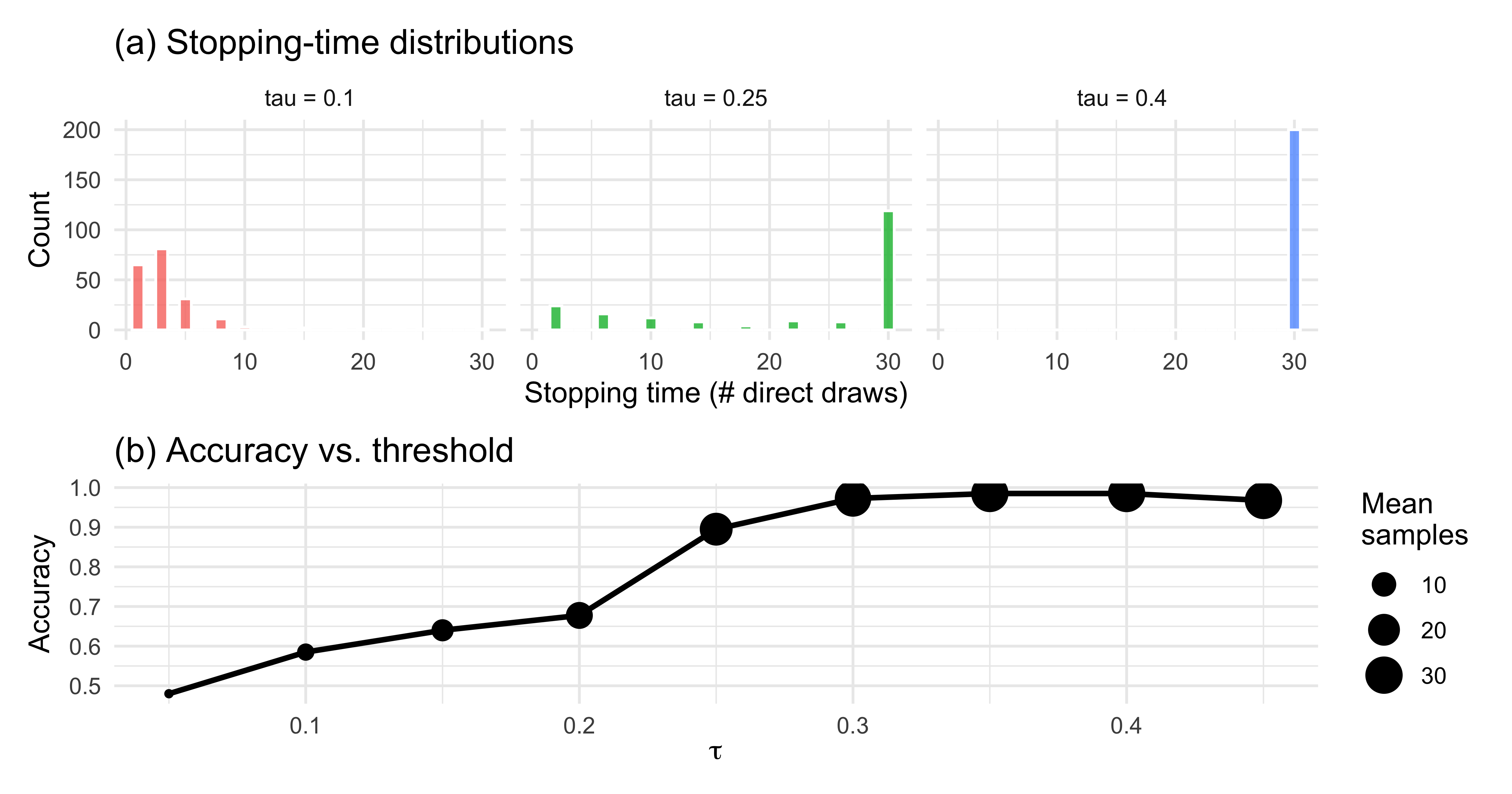
```{r ch11_threshold_viz, fig.height = 4.2}
# (a) Stopping-time distributions per tau
p_stop <- sim_threshold |>
  ggplot(aes(T, fill = tau_label)) +
  geom_histogram(binwidth = 1, colour = "white", alpha = 0.8) +
  facet_wrap(~tau_label, ncol = 3) +
  labs(x = "Stopping time (# direct draws)",
       y = "Count",
       title = "(a) Stopping-time distributions") +
  theme(legend.position = "none")

# (b) Accuracy vs. tau (sweep on a denser grid)
tau_sweep <- seq(0.05, 0.45, by = 0.05)
acc_df <- purrr::map_dfr(tau_sweep, function(tt) {
  s <- simulate_threshold_agent(tau = tt, n_trials = 400)
  tibble(tau = tt,
         accuracy    = mean(s$correct),
         mean_T      = mean(s$T))
})

p_acc <- acc_df |>
  ggplot(aes(tau, accuracy)) +
  geom_line(size = 1) +
  geom_point(aes(size = mean_T)) +
  scale_size_continuous(name = "Mean\nsamples") +
  labs(x = expression(tau), y = "Accuracy",
       title = "(b) Accuracy vs. threshold")

p_stop / p_acc
```
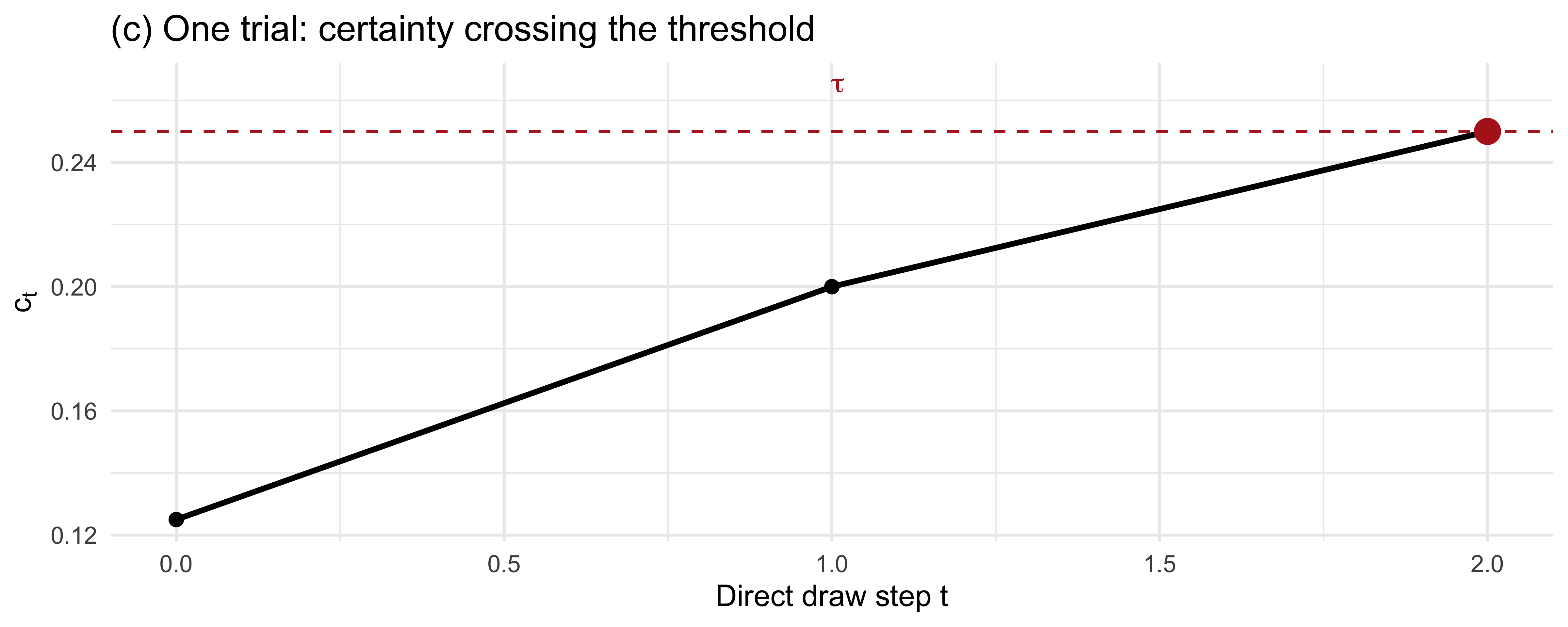
```{r ch11_threshold_trace, fig.height = 3.2}
# (c) Trial-trace: certainty evolving toward the threshold
set.seed(42)
trace_tau <- 0.25
alpha_t <- 0.5 + 1
beta_t  <- 0.5 + (3 - 1)
trace <- tibble(
  t       = 0,
  alpha_t = alpha_t,
  beta_t  = beta_t,
  c_t     = abs(alpha_t / (alpha_t + beta_t) - 0.5)
)
for (t in 1:20) {
  draw <- rbinom(1, 1, 0.75)
  alpha_t <- alpha_t + draw
  beta_t  <- beta_t + (1 - draw)
  trace <- bind_rows(trace, tibble(
    t = t,
    alpha_t = alpha_t, beta_t = beta_t,
    c_t = abs(alpha_t / (alpha_t + beta_t) - 0.5)
  ))
  if (abs(alpha_t / (alpha_t + beta_t) - 0.5) >= trace_tau) break
}
stop_t <- max(trace$t)

trace |>
  ggplot(aes(t, c_t)) +
  geom_line(size = 1) +
  geom_point(size = 2) +
  geom_hline(yintercept = trace_tau, linetype = "dashed", colour = "firebrick") +
  annotate("text", x = 1, y = trace_tau + 0.015,
           label = expression(tau), colour = "firebrick", hjust = 0) +
  annotate("point", x = stop_t, y = trace$c_t[trace$t == stop_t],
           colour = "firebrick", size = 4) +
  labs(x = "Direct draw step t", y = expression(c[t]),
       title = "(c) One trial: certainty crossing the threshold")
```
The patterns line up with intuition: a low $\tau$ produces short,
noisy, error-prone trials; a high $\tau$ produces longer, more accurate
trials with diminishing returns.
### Single-agent Stan model (soft threshold)
The hard rule above is unsuitable for HMC because it is
non-differentiable in $\tau$. We replace it with a logistic soft rule.
The likelihood then becomes a product of Bernoulli stop/continue
probabilities plus a Bernoulli for the final guess. Because the
direct-evidence sequence itself is a latent variable conditional only on
$T_i$ and the final $(\alpha, \beta)$, we pass the raw per-step draws
(reconstructed from the simulation) to Stan as data. In a real analysis
the modeller would either record these draws in the experiment or
marginalise over them.
```{r ch11_threshold_stan_data}
# Use the tau = 0.25 agent for fitting. Re-run the simulation but also
# record the sequence of draws for each trial.
simulate_threshold_agent_full <- function(tau, n_trials, max_samples = 30,
                                          true_theta = 0.7,
                                          social_k = 1, social_n = 3) {
  draws_list <- vector("list", n_trials)
  T_vec <- integer(n_trials)
  g_vec <- integer(n_trials)
  for (i in seq_len(n_trials)) {
    alpha_t <- 0.5 + social_k
    beta_t  <- 0.5 + (social_n - social_k)
    draws_i <- integer(0)
    t <- 0
    stopped <- FALSE
    while (!stopped && t < max_samples) {
      c_t <- abs(alpha_t / (alpha_t + beta_t) - 0.5)
      if (c_t >= tau && t >= 1) { stopped <- TRUE; break }
      t <- t + 1
      d <- rbinom(1, 1, true_theta)
      draws_i <- c(draws_i, d)
      alpha_t <- alpha_t + d
      beta_t  <- beta_t + (1 - d)
    }
    T_vec[i] <- t
    g_vec[i] <- as.integer(alpha_t > beta_t)
    draws_list[[i]] <- draws_i
  }
  list(T = T_vec, guess = g_vec, draws = draws_list)
}

sim_full <- simulate_threshold_agent_full(tau = 0.25, n_trials = 120)

# Flatten per-trial draws into a padded matrix (max T across trials)
T_max_obs <- max(sim_full$T)
draws_mat <- matrix(0L, nrow = length(sim_full$T), ncol = T_max_obs)
for (i in seq_along(sim_full$draws)) {
  if (sim_full$T[i] > 0) {
    draws_mat[i, 1:sim_full$T[i]] <- sim_full$draws[[i]]
  }
}

stan_data_A <- list(
  N        = length(sim_full$T),
  T_max    = T_max_obs,
  T        = sim_full$T,
  guess    = sim_full$guess,
  draws    = draws_mat,
  social_k = 1,
  social_n = 3,
  sigma_tau = 0.02
)
```
```{r ch11_threshold_stan_code}
ThresholdAgent_stan <- "
// Sample-or-Guess Agent with a soft certainty threshold.
// Single parameter: tau in (0, 0.5), the certainty threshold.
// The stop/continue decision is modelled with a logistic soft rule
// around tau with fixed slope sigma_tau.

data {
  int<lower=1> N;
  int<lower=1> T_max;
  array[N] int<lower=0, upper=T_max> T;
  array[N] int<lower=0, upper=1> guess;
  array[N, T_max] int<lower=0, upper=1> draws;
  int<lower=0> social_k;
  int<lower=0> social_n;
  real<lower=0> sigma_tau;
}

parameters {
  // tau ~ scaled Beta(2,2) on (0, 0.5)
  real<lower=0, upper=0.5> tau;
}

model {
  // Prior: Beta(2,2) on (0, 0.5) via change of variables -> tau * 2 ~ Beta(2,2)
  target += beta_lpdf(2 * tau | 2, 2) + log(2);

  for (i in 1:N) {
    real alpha_t = 0.5 + social_k;
    real beta_t  = 0.5 + (social_n - social_k);

    // Steps 1 .. T[i] - 1: the agent continued (soft prob of NOT stopping)
    // At step T[i]: the agent stopped (soft prob of stopping)
    // If T[i] == 0 (agent would stop before seeing any direct draw) we
    // only contribute the final guess.
    for (t in 1:T[i]) {
      int d = draws[i, t];
      alpha_t += d;
      beta_t  += (1 - d);
      real c_t = abs(alpha_t / (alpha_t + beta_t) - 0.5);
      real p_stop = inv_logit((c_t - tau) / sigma_tau);
      if (t < T[i]) {
        target += bernoulli_lpmf(0 | p_stop);  // continued
      } else {
        target += bernoulli_lpmf(1 | p_stop);  // stopped
      }
    }

    // Final guess given the posterior at stopping time
    {
      real alpha_final = 0.5 + social_k;
      real beta_final  = 0.5 + (social_n - social_k);
      for (t in 1:T[i]) {
        alpha_final += draws[i, t];
        beta_final  += (1 - draws[i, t]);
      }
      real p_blue = alpha_final / (alpha_final + beta_final);
      target += bernoulli_lpmf(guess[i] | p_blue);
    }
  }
}
"

write_stan_file(ThresholdAgent_stan,
                dir = "stan/",
                basename = "ch11_threshold_agent.stan")
```
```{r ch11_threshold_fit, results = "hide"}
mod_A <- cmdstan_model("stan/ch11_threshold_agent.stan", dir = "simmodels")

if (regenerate_simulations || !file.exists("simmodels/ch11_fit_A.rds")) {
  fit_A <- mod_A$sample(
    data = stan_data_A,
    seed = 123,
    chains = 2,
    parallel_chains = 2,
    iter_warmup = 500,
    iter_sampling = 500,
    refresh = 0
  )
  fit_A$save_object("simmodels/ch11_fit_A.rds")
} else {
  fit_A <- readRDS("simmodels/ch11_fit_A.rds")
}
```
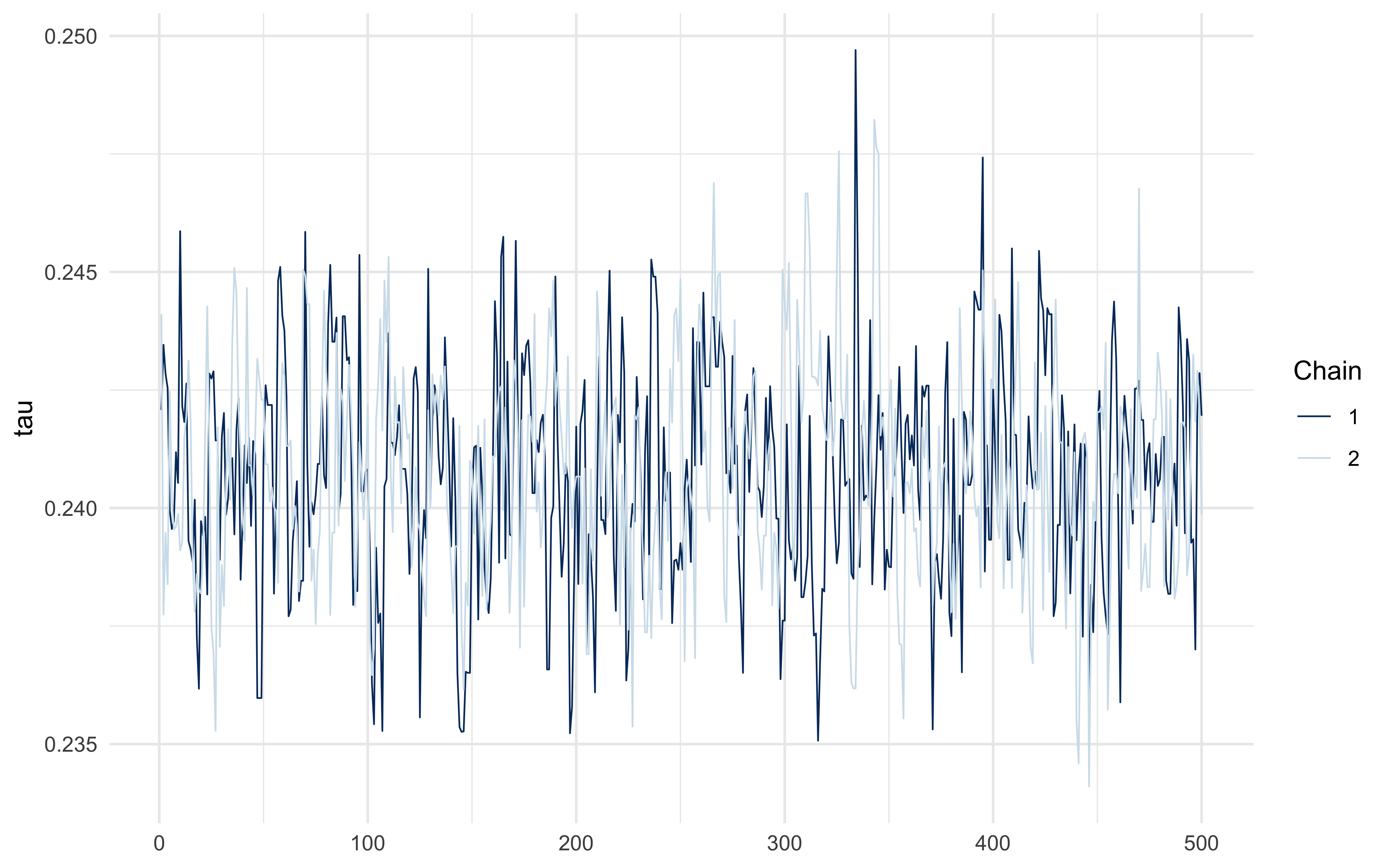
```{r ch11_threshold_diagnostics}
fit_A$summary("tau")
mcmc_trace(fit_A$draws("tau"))
```
The posterior should concentrate near the simulated $\tau = 0.25$ — but
with meaningful width, because the soft rule trades off slope ($\sigma_\tau$)
against threshold location. The hard-rule identifiability limit is an
interesting project question.
## Section B: Adaptive-Weight Agent
### Conceptual motivation
The WBA of Ch. 10 commits at $t = 0$ to fixed weights $w_d$ and $w_s$ on
direct and social evidence, and carries them through the entire
experiment. But a sensible agent should update those weights: if social
tips keep steering them wrong, they should trust the social source
*less*; if direct observations keep being misleading (a noisy sensor,
say), they should trust themselves less. This turns the static WBA into
a *learning* model, and makes contact with the reinforcement-learning
framing of Ch. 3 — except that the thing being learned is not a value,
but a meta-parameter governing how two information streams are
combined. The resulting agent is Bayesian *within* a trial (it still
integrates evidence via the Beta-Binomial posterior) but RL-like
*across* trials (it updates weights from prediction errors).
This extension also provides a mechanistic story for why real agents
might look like different static WBAs at different points in an
experiment: they are one agent whose weights have drifted.
### Mathematical formalization
On each trial $t$, the two sources make independent predictions of the
correct colour:
$$p_{d,t} = \frac{\alpha_{d,t}}{\alpha_{d,t} + \beta_{d,t}},
\qquad
p_{s,t} = \frac{\alpha_{s,t}}{\alpha_{s,t} + \beta_{s,t}},$$
where $(\alpha_{d,t}, \beta_{d,t})$ is the posterior from *only* the
direct evidence on trial $t$, and $(\alpha_{s,t}, \beta_{s,t})$ is the
posterior from *only* the social evidence. The agent's combined
posterior (and its guess) uses the WBA combination with *current*
weights $w_{d,t}, w_{s,t}$:
$$\alpha_t = 0.5 + w_{d,t} k_{d,t} + w_{s,t} k_{s,t}, \qquad
\beta_t = 0.5 + w_{d,t} (n_{d,t} - k_{d,t}) + w_{s,t} (n_{s,t} - k_{s,t}).$$
After feedback $y_t \in \{0, 1\}$ on the correct colour, each source's
per-trial prediction error is
$$\delta_{d,t} = y_t - p_{d,t}, \qquad \delta_{s,t} = y_t - p_{s,t}.$$
The weights update on the log scale (to keep them positive) by a delta
rule that rewards the source that predicted better:
$$\log w_{d,t+1} = \log w_{d,t} + \eta\,(|\delta_{s,t}| - |\delta_{d,t}|),$$
$$\log w_{s,t+1} = \log w_{s,t} + \eta\,(|\delta_{d,t}| - |\delta_{s,t}|).$$
Parameters: learning rate $\eta \in (0, 1)$ and initial log-weights
$\log w_{d,0}, \log w_{s,0}$.
### R forward simulation
```{r ch11_adaptive_agent_fn}
# Generate a stream of trials with specified direct/social reliability.
# direct_reliability / social_reliability: probability that the source
# points to the correct colour on any given trial.
make_trial_stream <- function(n_trials, direct_reliability,
                              social_reliability, n_d = 4, n_s = 3) {
  purrr::map_dfr(seq_len(n_trials), function(i) {
    correct <- rbinom(1, 1, 0.5)  # truth randomly blue/red
    # Each direct draw agrees with the truth with prob direct_reliability
    k_d <- rbinom(1, n_d, if (correct == 1) direct_reliability
                          else 1 - direct_reliability)
    k_s <- rbinom(1, n_s, if (correct == 1) social_reliability
                          else 1 - social_reliability)
    tibble(trial = i, correct = correct,
           k_d = k_d, n_d = n_d, k_s = k_s, n_s = n_s)
  })
}

simulate_adaptive_agent <- function(eta, w_d0, w_s0, trial_stream,
                                    alpha0 = 0.5, beta0 = 0.5) {
  w_d <- w_d0
  w_s <- w_s0
  out <- vector("list", nrow(trial_stream))
  for (i in seq_len(nrow(trial_stream))) {
    tr <- trial_stream[i, ]
    # Source-specific posteriors
    alpha_d <- alpha0 + tr$k_d
    beta_d  <- beta0  + (tr$n_d - tr$k_d)
    alpha_s <- alpha0 + tr$k_s
    beta_s  <- beta0  + (tr$n_s - tr$k_s)
    p_d <- alpha_d / (alpha_d + beta_d)
    p_s <- alpha_s / (alpha_s + beta_s)

    # Combined WBA posterior with current weights
    alpha_c <- alpha0 + w_d * tr$k_d + w_s * tr$k_s
    beta_c  <- beta0  + w_d * (tr$n_d - tr$k_d) + w_s * (tr$n_s - tr$k_s)
    p_c     <- alpha_c / (alpha_c + beta_c)
    guess   <- rbinom(1, 1, p_c)

    # Delta rule on log-weights
    y <- tr$correct
    d_d <- abs(y - p_d)
    d_s <- abs(y - p_s)
    w_d <- exp(log(w_d) + eta * (d_s - d_d))
    w_s <- exp(log(w_s) + eta * (d_d - d_s))

    out[[i]] <- tibble(trial = tr$trial, correct = y, guess = guess,
                       p_c = p_c, w_d = w_d, w_s = w_s,
                       k_d = tr$k_d, n_d = tr$n_d,
                       k_s = tr$k_s, n_s = tr$n_s)
  }
  bind_rows(out)
}

# Three regimes
set.seed(7)
regimes <- tibble(
  regime = c("direct more reliable", "social more reliable", "equally reliable"),
  rel_d  = c(0.85, 0.55, 0.75),
  rel_s  = c(0.55, 0.85, 0.75)
)

sim_adapt <- purrr::pmap_dfr(regimes, function(regime, rel_d, rel_s) {
  stream <- make_trial_stream(n_trials = 120,
                              direct_reliability = rel_d,
                              social_reliability = rel_s)
  simulate_adaptive_agent(eta = 0.2, w_d0 = 1, w_s0 = 1, trial_stream = stream) |>
    mutate(regime = regime)
})
```
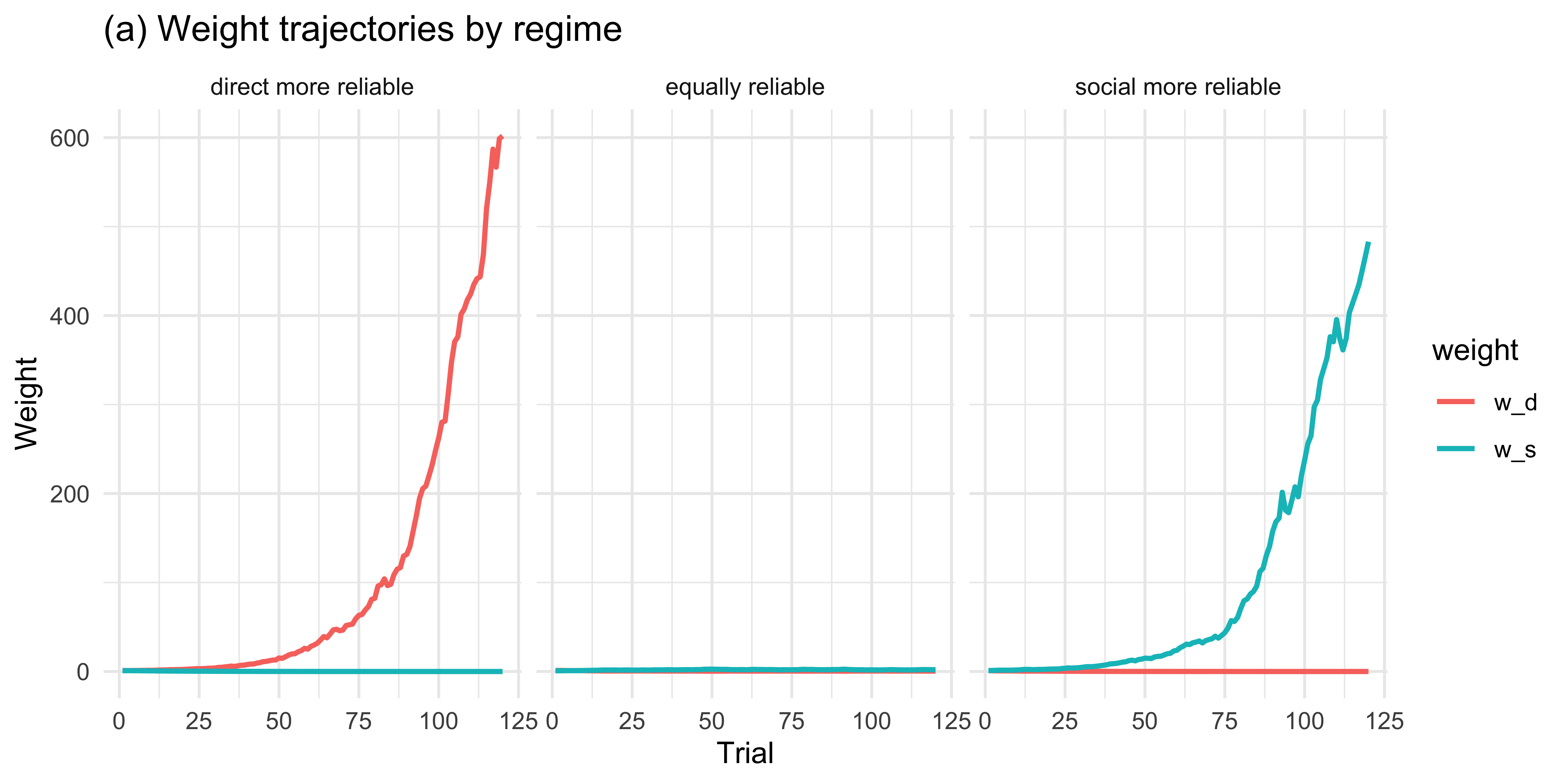
### Visualisations
```{r ch11_adaptive_viz_a, fig.height = 4}
sim_adapt |>
  pivot_longer(c(w_d, w_s), names_to = "weight", values_to = "value") |>
  ggplot(aes(trial, value, colour = weight)) +
  geom_line(size = 0.9) +
  facet_wrap(~regime) +
  labs(title = "(a) Weight trajectories by regime",
       y = "Weight", x = "Trial")
```
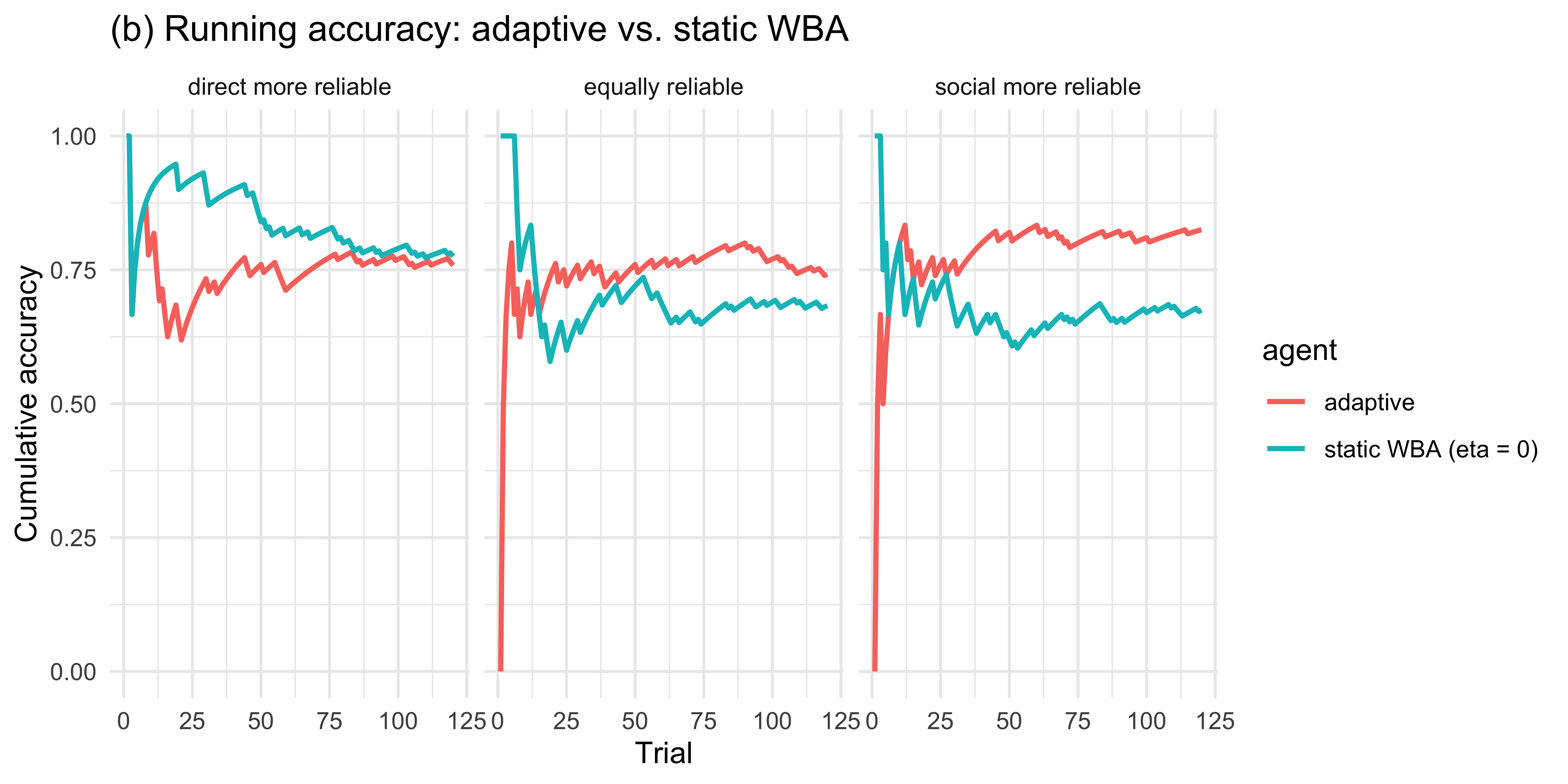
```{r ch11_adaptive_viz_b, fig.height = 4}
# Compare adaptive agent vs. static WBA (w_d = w_s = 1) on accuracy
set.seed(8)
compare_df <- purrr::pmap_dfr(regimes, function(regime, rel_d, rel_s) {
  stream <- make_trial_stream(n_trials = 120,
                              direct_reliability = rel_d,
                              social_reliability = rel_s)
  adaptive <- simulate_adaptive_agent(0.2, 1, 1, stream) |>
    mutate(agent = "adaptive")
  static <- simulate_adaptive_agent(0.0, 1, 1, stream) |>
    mutate(agent = "static WBA (eta = 0)")
  bind_rows(adaptive, static) |> mutate(regime = regime)
})

compare_df |>
  mutate(correct_guess = as.integer(guess == correct)) |>
  group_by(regime, agent, trial) |>
  summarise(acc = mean(correct_guess), .groups = "drop") |>
  group_by(regime, agent) |>
  mutate(running_acc = cumsum(acc) / seq_along(acc)) |>
  ggplot(aes(trial, running_acc, colour = agent)) +
  geom_line(size = 0.9) +
  facet_wrap(~regime) +
  labs(title = "(b) Running accuracy: adaptive vs. static WBA",
       y = "Cumulative accuracy", x = "Trial")
```
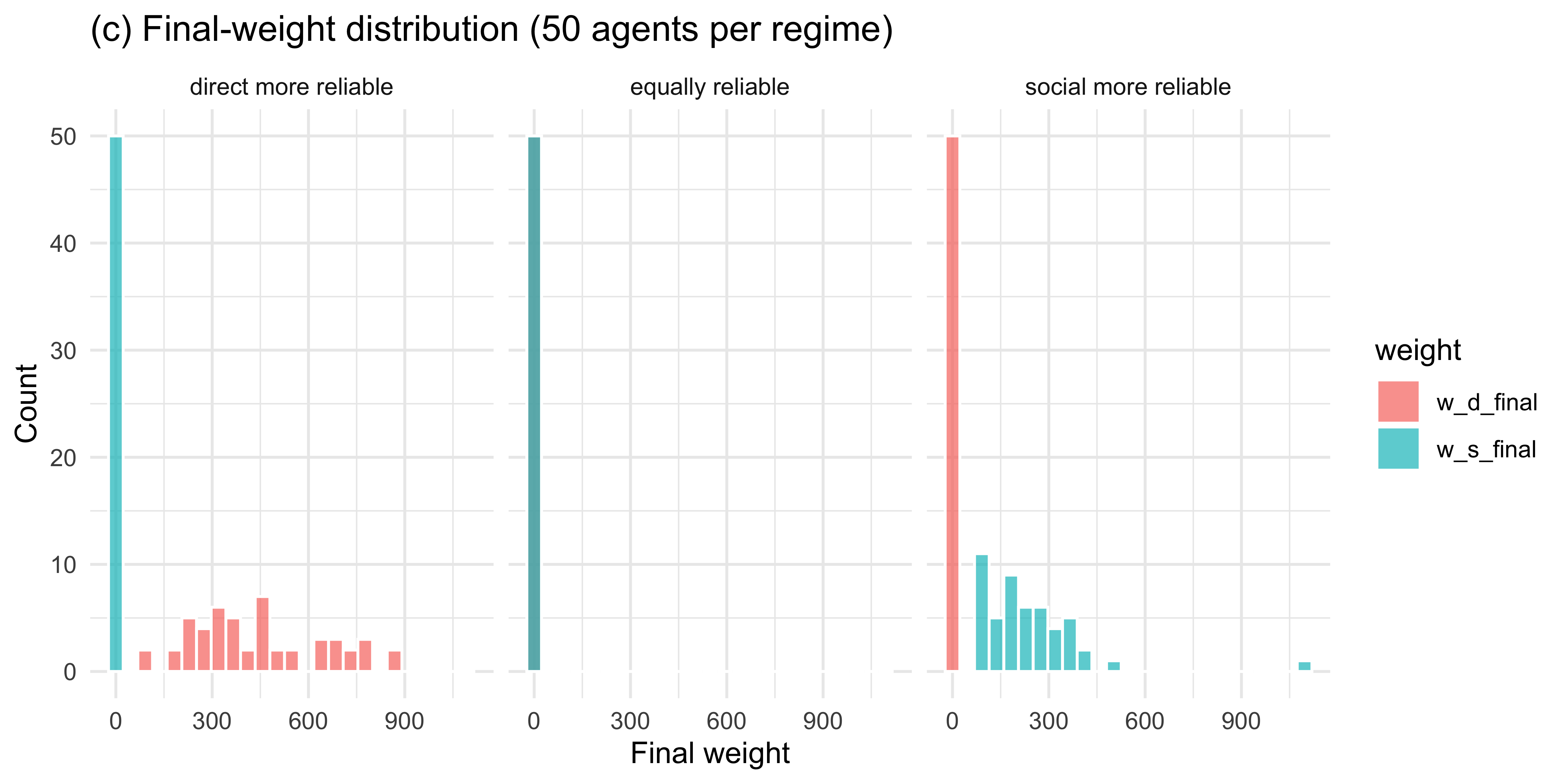
```{r ch11_adaptive_viz_c, fig.height = 4}
# Final-weight distribution across 50 simulated agents per regime
set.seed(9)
final_df <- purrr::pmap_dfr(regimes, function(regime, rel_d, rel_s) {
  purrr::map_dfr(1:50, function(a) {
    stream <- make_trial_stream(120, rel_d, rel_s)
    res <- simulate_adaptive_agent(0.2, 1, 1, stream)
    tibble(agent_id = a, regime = regime,
           w_d_final = tail(res$w_d, 1),
           w_s_final = tail(res$w_s, 1))
  })
})

final_df |>
  pivot_longer(c(w_d_final, w_s_final), names_to = "weight", values_to = "value") |>
  ggplot(aes(value, fill = weight)) +
  geom_histogram(bins = 25, alpha = 0.7, position = "identity", colour = "white") +
  facet_wrap(~regime) +
  labs(title = "(c) Final-weight distribution (50 agents per regime)",
       x = "Final weight", y = "Count")
```
Across 50 simulated agents the weights track the true reliability
asymmetry: when direct evidence is more reliable, $w_d$ grows and $w_s$
shrinks; the pattern reverses when social evidence is more reliable;
and when the two are matched, weights drift modestly in either
direction without systematic asymmetry.
### Single-agent Stan model
```{r ch11_adaptive_stan_data}
# Fit to one direct-more-reliable agent
set.seed(11)
stream_fit <- make_trial_stream(120, direct_reliability = 0.85,
                                 social_reliability = 0.55)
sim_fit <- simulate_adaptive_agent(0.2, 1, 1, stream_fit)

stan_data_B <- list(
  N       = nrow(sim_fit),
  guess   = sim_fit$guess,
  correct = sim_fit$correct,
  k_d     = sim_fit$k_d,
  n_d     = sim_fit$n_d,
  k_s     = sim_fit$k_s,
  n_s     = sim_fit$n_s
)
```
```{r ch11_adaptive_stan_code}
AdaptiveAgent_stan <- "
// Adaptive-Weight Agent.
// Parameters: eta (learning rate), log w_d0, log w_s0 (initial log-weights).
// Weights are updated across trials by a delta rule on log-weights using
// per-source absolute prediction errors against the feedback.

data {
  int<lower=1> N;
  array[N] int<lower=0, upper=1> guess;
  array[N] int<lower=0, upper=1> correct;
  array[N] int<lower=0> k_d;
  array[N] int<lower=0> n_d;
  array[N] int<lower=0> k_s;
  array[N] int<lower=0> n_s;
}

parameters {
  real<lower=0, upper=1> eta;
  real log_w_d0;
  real log_w_s0;
}

transformed parameters {
  vector[N] p_c;
  {
    real log_w_d = log_w_d0;
    real log_w_s = log_w_s0;
    for (i in 1:N) {
      real w_d = exp(log_w_d);
      real w_s = exp(log_w_s);

      real alpha_d = 0.5 + k_d[i];
      real beta_d  = 0.5 + (n_d[i] - k_d[i]);
      real alpha_s = 0.5 + k_s[i];
      real beta_s  = 0.5 + (n_s[i] - k_s[i]);
      real p_d = alpha_d / (alpha_d + beta_d);
      real p_s = alpha_s / (alpha_s + beta_s);

      real alpha_c = 0.5 + w_d * k_d[i] + w_s * k_s[i];
      real beta_c  = 0.5 + w_d * (n_d[i] - k_d[i]) + w_s * (n_s[i] - k_s[i]);
      p_c[i] = alpha_c / (alpha_c + beta_c);

      real d_d = abs(correct[i] - p_d);
      real d_s = abs(correct[i] - p_s);
      log_w_d += eta * (d_s - d_d);
      log_w_s += eta * (d_d - d_s);
    }
  }
}

model {
  target += beta_lpdf(eta | 2, 5);
  target += normal_lpdf(log_w_d0 | 0, 1);
  target += normal_lpdf(log_w_s0 | 0, 1);

  target += bernoulli_lpmf(guess | p_c);
}
"

write_stan_file(AdaptiveAgent_stan,
                dir = "stan/",
                basename = "ch11_adaptive_agent.stan")
```
```{r ch11_adaptive_fit, results = "hide"}
mod_B <- cmdstan_model("stan/ch11_adaptive_agent.stan", dir = "simmodels")

if (regenerate_simulations || !file.exists("simmodels/ch11_fit_B.rds")) {
  fit_B <- mod_B$sample(
    data = stan_data_B,
    seed = 321,
    chains = 2,
    parallel_chains = 2,
    iter_warmup = 500,
    iter_sampling = 500,
    refresh = 0
  )
  fit_B$save_object("simmodels/ch11_fit_B.rds")
} else {
  fit_B <- readRDS("simmodels/ch11_fit_B.rds")
}
```
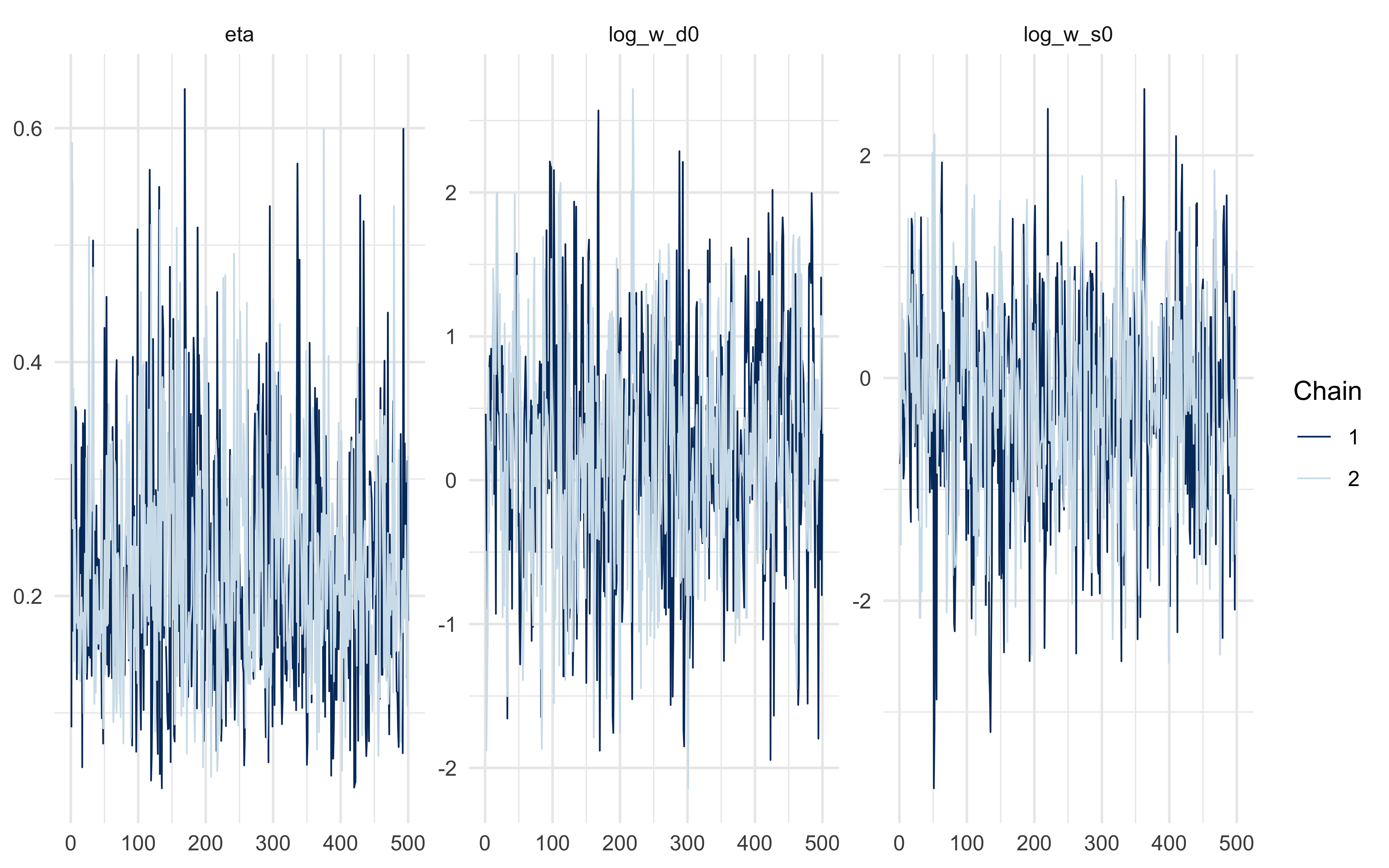
```{r ch11_adaptive_diagnostics}
fit_B$summary(c("eta", "log_w_d0", "log_w_s0"))
mcmc_trace(fit_B$draws(c("eta", "log_w_d0", "log_w_s0")))
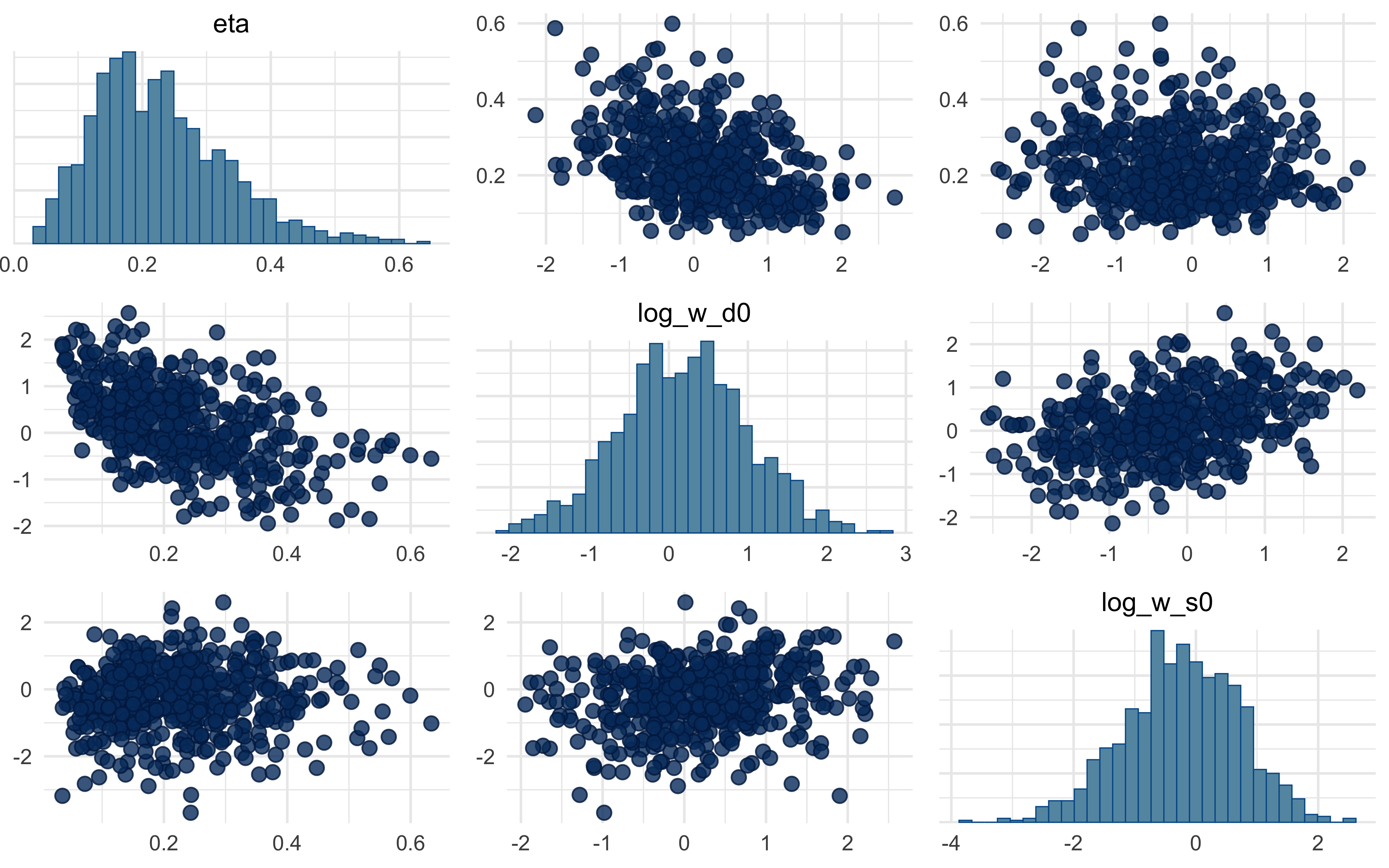
mcmc_pairs(fit_B$draws(c("eta", "log_w_d0", "log_w_s0")))
```
A note on what you will almost certainly see in the pairs plot: a strong
ridge between $\eta$ and the initial log-weights. This is not a bug — it
is structural. A small $\eta$ with strongly asymmetric starting weights
produces similar behaviour to a large $\eta$ with symmetric starts,
because both paths arrive at similar *effective* weights by the end of
the trial stream. We flag this rather than hide it: demonstrating and
resolving the non-identifiability (via informative priors, via
parameter-informative experimental designs that force the weights to
change across blocks, or via multilevel partial pooling) is a natural
student project.
## Closing
The Bayesian-cognition hypothesis is a family of models, not a single
commitment. Once an agent represents beliefs as probability
distributions and integrates evidence by Bayes' rule, many further
modelling choices remain open: when to stop sampling, how to weight
sources, whether those weights themselves are learned, what the
observation model looks like. The sample-or-guess and adaptive-weight
agents above are natural sequential extensions of the Ch. 10 family and
make good starting points for student projects — a full validation
battery (parameter recovery, SBC, model comparison, multilevel pooling)
on either model is left as an exercise in applying the workflow you
have already learned.