Chapter 8 Bonus chapter: Additional models developed by students
8.1 Additional models
Additional models that have been developed by previous students:
8.1.3 Memory agent with exponential memory decay (rate)
Memory = alpha * memory + (1 - alpha) * otherChoice
8.1.4 Memory agent with exponential memory decay (exponential)
The agent uses a weighted memory store, where previous choices are weighted by a factor based on how far back in the past they were made, represented by power. The agent first creates a vector of weights for each of the previous choices based on their position in the memory store and the power value. This model implements exponential decay of memory, according to a power law. Specifically, the opposing agent’s choices up to the present trial are encoded as 1’s and -1’s. The choices are weighted, and then summed. So, on trial i, the memory of the previous trial j is given a weight corresponding to j^(-1). Higher values of j correspond to earlier trials, with j = 1 being the most recent. Then a choice is made based on this weight according to the following formula:
Theta = inv_logit(alpha + beta * weightedMemory)
[N.B. really poor parameter recovery]
8.1.5 Memory agent with exponential memory decay, but separate memory for wins and losses
[N.B. really poor parameter recovery]
8.4 Generate data
[MISSING: EXPLAIN THE MODEL STEP BY STEP]
[MISSING: PARALLELIZE AND MAKE IT MORE SIMILAR TO PREVIOUS DATASETS]
8.5 Sanity check for the data
d <- d %>% group_by(agent, strategy) %>% mutate(
  nextChoice = lead(choice),
  prevWin = lag(win),
  prevLose = lag(lose),
  cumulativerate = cumsum(choice) / seq_along(choice),
  performance = cumsum(feedback) / seq_along(feedback)
) %>% subset(complete.cases(d)) %>% subset(trial > 1)

p1 <- ggplot(d, aes(trial, cumulativerate, group = agent, color = agent)) +
  geom_line() +
  geom_hline(yintercept = 0.5, linetype = "dashed") + ylim(0,1) + theme_classic() + facet_wrap(.~strategy)
p1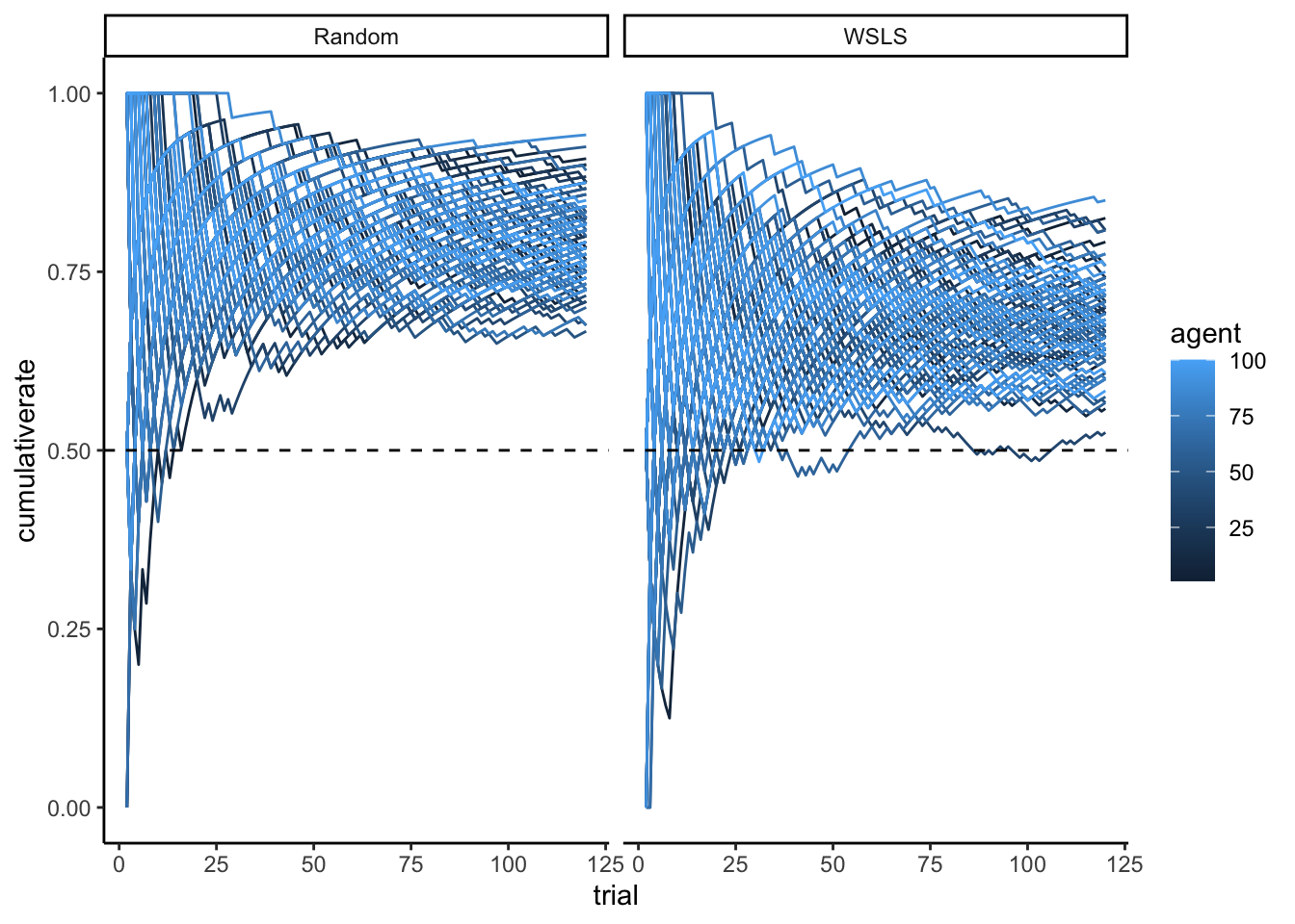
p2a <- ggplot(subset(d, strategy == "Random"), aes(trial, 1 - performance, group = agent, color = agent)) +
  geom_line() +
  geom_hline(yintercept = 0.5, linetype = "dashed") + ylim(0,1) + theme_classic()
p2b <- ggplot(subset(d, strategy == "WSLS"), aes(trial, performance, group = agent, color = agent)) +
  geom_line() +
  geom_hline(yintercept = 0.5, linetype = "dashed") + ylim(0,1) + theme_classic()
library(patchwork)
p2a + p2b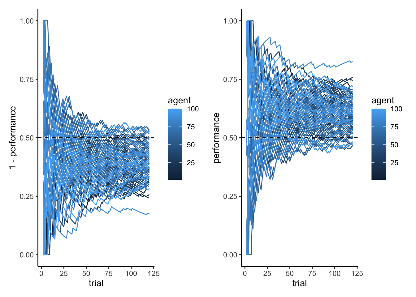
8.6 More sanity check
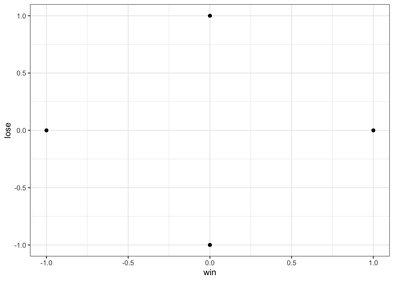
## Checking lose/win do determine choice
d %>% subset(strategy == "WSLS") %>%
  mutate(nextChoice = lead(choice)) %>%
  group_by(agent, win, lose) %>%
  summarize(heads = mean(nextChoice)) %>%
  ggplot(aes(win, heads)) +
       geom_point() +
       theme_bw() +
  facet_wrap(~lose)
## `summarise()` has grouped output by 'agent', 'win'. You can override using the
## `.groups` argument.## Warning: Removed 100 rows containing missing values (`geom_point()`).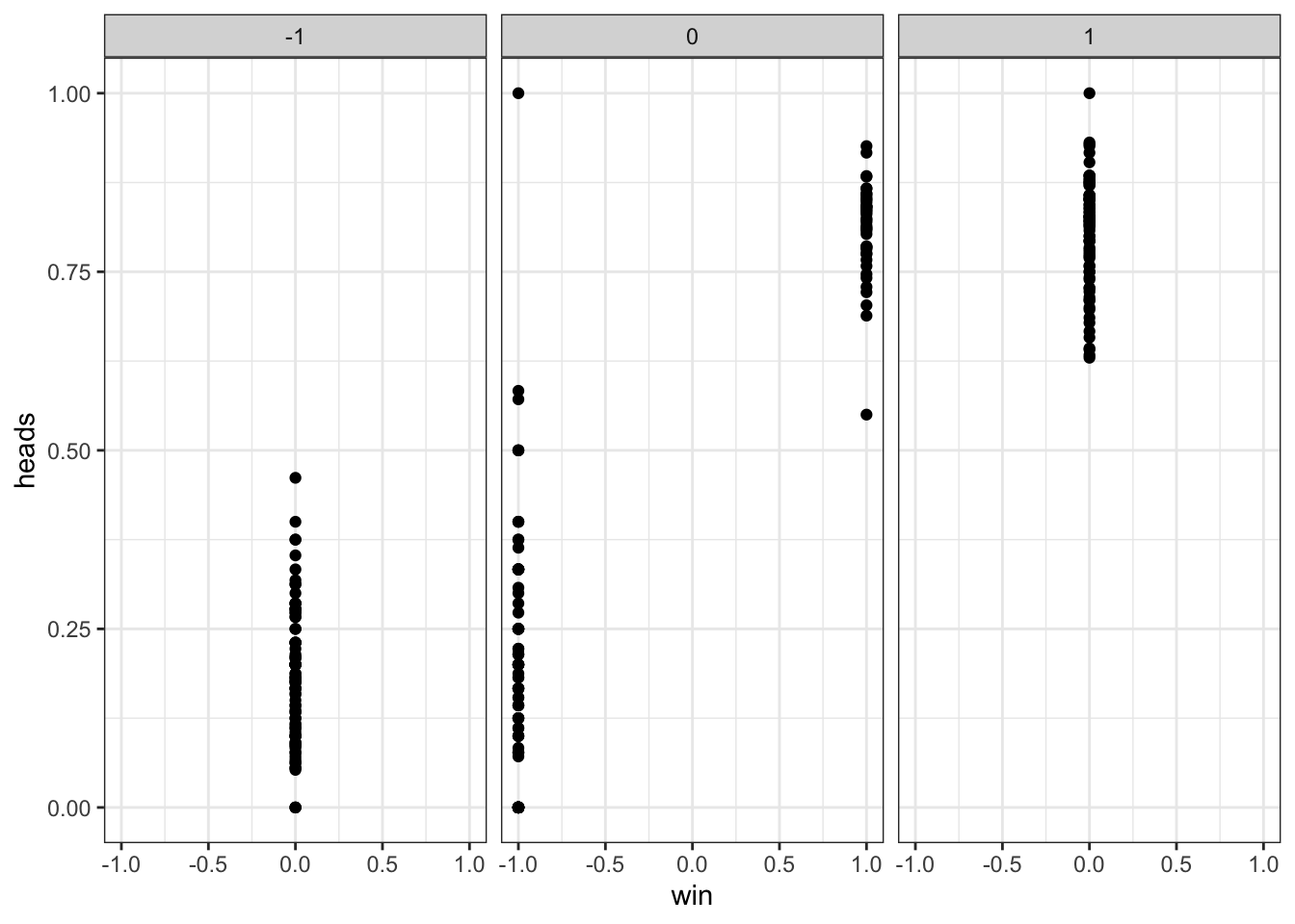
8.8 Create the model
[MISSING: MORE MEANINGFUL PREDICTIONS, BASED ON THE 4 SCENARIOS]
stan_wsls_model <- "

functions{
  real normal_lb_rng(real mu, real sigma, real lb) {
    real p = normal_cdf(lb | mu, sigma);  // cdf for bounds
    real u = uniform_rng(p, 1);
    return (sigma * inv_Phi(u)) + mu;  // inverse cdf for value
  }
}

data {
 int<lower = 1> trials;
 array[trials] int h;
 vector[trials] win;
 vector[trials] lose;
}

parameters {
  real alpha;
  real winB;
  real loseB;
}

model {
  target += normal_lpdf(alpha | 0, .3);
  target += normal_lpdf(winB | 1, 1);
  target += normal_lpdf(loseB | 1, 1);
  target += bernoulli_logit_lpmf(h | alpha + winB * win + loseB * lose);
}

generated quantities{
   real alpha_prior;
   real winB_prior;
   real loseB_prior;
   array[trials] int prior_preds;
   array[trials] int posterior_preds;
   vector[trials] log_lik;

   alpha_prior = normal_rng(0, 1);
   winB_prior = normal_rng(0, 1);
   loseB_prior = normal_rng(0, 1);

   prior_preds = bernoulli_rng(inv_logit(winB_prior * win +  loseB_prior * lose));
   posterior_preds = bernoulli_rng(inv_logit(winB * win +  loseB * lose));

    for (t in 1:trials){
      log_lik[t] = bernoulli_logit_lpmf(h[t] | winB * win +  loseB * lose);
    }

}

"

write_stan_file(
  stan_wsls_model,
  dir = "stan/",
  basename = "W8_WSLS.stan")
## [1] "/Users/au209589/Dropbox/Teaching/AdvancedCognitiveModeling23_book/stan/W8_WSLS.stan"file <- file.path("stan/W8_WSLS.stan")
mod_wsls_simple <- cmdstan_model(file,
cpp_options = list(stan_threads = TRUE),
stanc_options = list("O1"),
pedantic = TRUE)
samples_wsls_simple <- mod_wsls_simple$sample(
data = data_wsls_simple,
seed = 123,
chains = 2,
parallel_chains = 2,
threads_per_chain = 2,
iter_warmup = 2000,
iter_sampling = 2000,
refresh = 1000,
max_treedepth = 20,
adapt_delta = 0.99,
)## Running MCMC with 2 parallel chains, with 2 thread(s) per chain...
##
## Chain 1 Iteration: 1 / 4000 [ 0%] (Warmup)
## Chain 1 Iteration: 1000 / 4000 [ 25%] (Warmup)
## Chain 1 Iteration: 2000 / 4000 [ 50%] (Warmup)
## Chain 1 Iteration: 2001 / 4000 [ 50%] (Sampling)
## Chain 2 Iteration: 1 / 4000 [ 0%] (Warmup)
## Chain 2 Iteration: 1000 / 4000 [ 25%] (Warmup)
## Chain 2 Iteration: 2000 / 4000 [ 50%] (Warmup)
## Chain 2 Iteration: 2001 / 4000 [ 50%] (Sampling)
## Chain 1 Iteration: 3000 / 4000 [ 75%] (Sampling)
## Chain 2 Iteration: 3000 / 4000 [ 75%] (Sampling)
## Chain 1 Iteration: 4000 / 4000 [100%] (Sampling)
## Chain 2 Iteration: 4000 / 4000 [100%] (Sampling)
## Chain 1 finished in 0.6 seconds.
## Chain 2 finished in 0.6 seconds.
##
## Both chains finished successfully.
## Mean chain execution time: 0.6 seconds.
## Total execution time: 0.8 seconds.8.9 Basic assessment
## # A tibble: 364 × 10
##    variable            mean   median    sd   mad      q5     q95  rhat ess_bulk ess_tail
##    <chr>              <dbl>    <dbl> <dbl> <dbl>   <dbl>   <dbl> <dbl>    <dbl>    <dbl>
##  1 lp__            -7.23e+1 -7.20e+1 1.26  1.04  -74.8   -71.0    1.00    1537.    2227.
##  2 alpha           -5.53e-2 -5.34e-2 0.199 0.200  -0.389   0.265  1.00    2359.    2142.
##  3 winB             1.02e+0  1.01e+0 0.297 0.304   0.547   1.52   1.00    2311.    2347.
##  4 loseB            1.10e+0  1.09e+0 0.322 0.311   0.589   1.65   1.00    2208.    2225.
##  5 alpha_prior     -1.14e-2 -5.82e-3 0.983 0.959  -1.66    1.57   1.00    4099.    4033.
##  6 winB_prior      -1.96e-2 -2.65e-2 0.999 0.996  -1.63    1.67   1.00    4182.    3530.
##  7 loseB_prior      1.86e-4 -5.70e-3 1.01  1.02   -1.65    1.67   1.00    3953.    3659.
##  8 prior_preds[1]   5.05e-1  1   e+0 0.500 0       0       1      1.00    3797.      NA
##  9 prior_preds[2]   5.06e-1  1   e+0 0.500 0       0       1      1.00    4120.      NA
## 10 prior_preds[3]   5.08e-1  1   e+0 0.500 0       0       1      1.00    3941.      NA
## # ℹ 354 more rows
# Extract posterior samples and include sampling of the prior:
draws_df <- as_draws_df(samples_wsls_simple$draws())
# Now let's plot the density for theta (prior and posterior)
ggplot(draws_df) +
geom_density(aes(alpha), fill = "blue", alpha = 0.3) +
geom_density(aes(alpha_prior), fill = "red", alpha = 0.3) +
geom_vline(xintercept = d_a$alpha[1]) +
xlab("Rate") +
ylab("Posterior Density") +
theme_classic()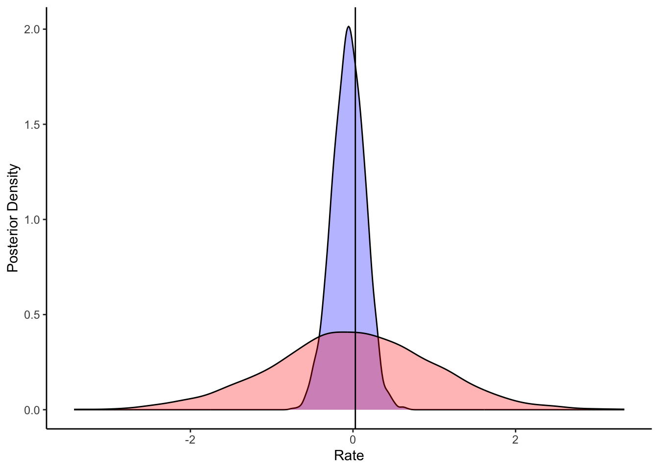
ggplot(draws_df) +
  geom_density(aes(winB), fill = "blue", alpha = 0.3) +
  geom_density(aes(winB_prior), fill = "red", alpha = 0.3) +
  geom_vline(xintercept = d_a$betaWin[1]) +
  xlab("Rate") +
  ylab("Posterior Density") +
  theme_classic()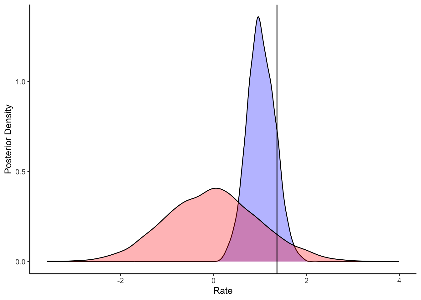
ggplot(draws_df) +
  geom_density(aes(loseB), fill = "blue", alpha = 0.3) +
  geom_density(aes(loseB_prior), fill = "red", alpha = 0.3) +
  geom_vline(xintercept = d_a$betaLose[1]) +
  xlab("Rate") +
  ylab("Posterior Density") +
  theme_classic()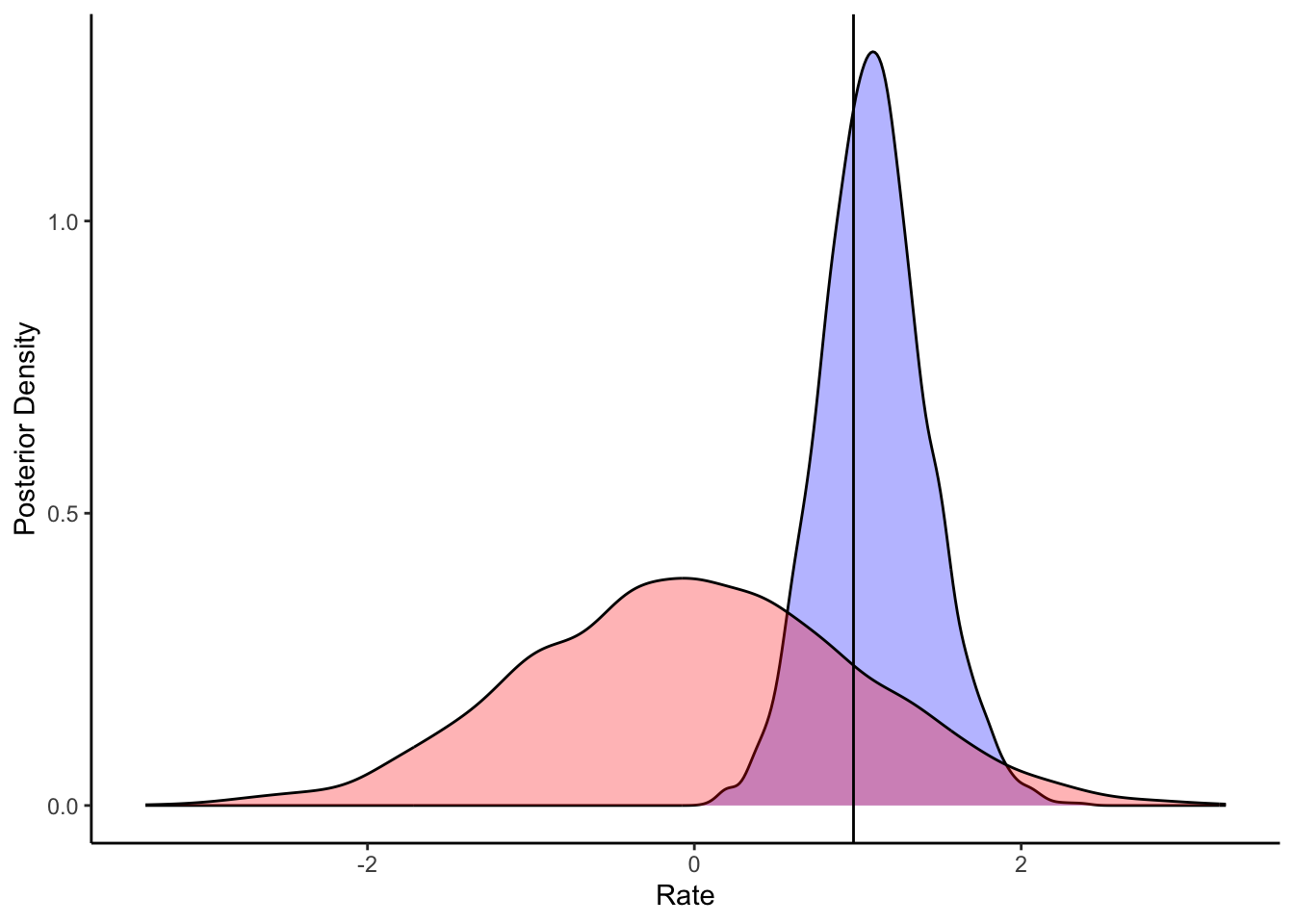
[MISSING: FULL PARAMETER RECOVERY]
8.10 Create multilevel data
## Now multilevel model
d_wsls1 <- d %>% subset(strategy == "WSLS") %>%
  subset(select = c(agent, choice)) %>%
  mutate(row = row_number()) %>%
  pivot_wider(names_from = agent, values_from = choice)
d_wsls2 <- d %>% subset(strategy == "WSLS") %>%
  subset(select = c(agent, prevWin)) %>%
  mutate(row = row_number()) %>%
  pivot_wider(names_from = agent, values_from = prevWin)
d_wsls3 <- d %>% subset(strategy == "WSLS") %>%
  subset(select = c(agent, prevLose)) %>%
  mutate(row = row_number()) %>%
  pivot_wider(names_from = agent, values_from = prevLose)

## Create the data
data_wsls <- list(
  trials = trials - 1,
  agents = agents,
  h = as.matrix(d_wsls1[,2:(agents + 1)]),
  win = as.matrix(d_wsls2[,2:(agents + 1)]),
  lose = as.matrix(d_wsls3[,2:(agents + 1)])
)
8.11 Create the model
[MISSING: ADD BIAS]
[MISSING: BETTER PREDICTIONS BASED ON 4 SCENARIOS]
stan_wsls_ml_model <- "
functions{
  real normal_lb_rng(real mu, real sigma, real lb) {
    real p = normal_cdf(lb | mu, sigma);  // cdf for bounds
    real u = uniform_rng(p, 1);
    return (sigma * inv_Phi(u)) + mu;  // inverse cdf for value
  }
}

// The input (data) for the model.
data {
 int<lower = 1> trials;
 int<lower = 1> agents;
 array[trials, agents] int h;
 array[trials, agents] real win;
 array[trials, agents] real lose;
}

parameters {
  real winM;
  real loseM;
  vector<lower = 0>[2] tau;
  matrix[2, agents] z_IDs;
  cholesky_factor_corr[2] L_u;
}

transformed parameters {
  matrix[agents,2] IDs;
  IDs = (diag_pre_multiply(tau, L_u) * z_IDs)';
 }

model {
  target += normal_lpdf(winM | 0, 1);
  target += normal_lpdf(tau[1] | 0, .3)  -
    normal_lccdf(0 | 0, .3);
  target += normal_lpdf(loseM | 0, .3);
  target += normal_lpdf(tau[2] | 0, .3)  -
    normal_lccdf(0 | 0, .3);
  target += lkj_corr_cholesky_lpdf(L_u | 2);

  target += std_normal_lpdf(to_vector(z_IDs));

  for (i in 1:agents)
    target += bernoulli_logit_lpmf(h[,i] | to_vector(win[,i]) * (winM + IDs[i,1]) +  to_vector(lose[,i]) * (loseM + IDs[i,2]));
}

generated quantities{
   real winM_prior;
   real<lower=0> winSD_prior;
   real loseM_prior;
   real<lower=0> loseSD_prior;

   real win_prior;
   real lose_prior;

   array[trials,agents] int<lower=0, upper = trials> prior_preds;
   array[trials,agents] int<lower=0, upper = trials> posterior_preds;

   array[trials, agents] real log_lik;


   winM_prior = normal_rng(0,1);
   winSD_prior = normal_lb_rng(0,0.3,0);
   loseM_prior = normal_rng(0,1);
   loseSD_prior = normal_lb_rng(0,0.3,0);

   win_prior = normal_rng(winM_prior, winSD_prior);
   lose_prior = normal_rng(loseM_prior, loseSD_prior);

   for (i in 1:agents){
      prior_preds[,i] = binomial_rng(trials, inv_logit(to_vector(win[,i]) * (win_prior) +  to_vector(lose[,i]) * (lose_prior)));
      posterior_preds[,i] = binomial_rng(trials, inv_logit(to_vector(win[,i]) * (winM + IDs[i,1]) +  to_vector(lose[,i]) * (loseM + IDs[i,2])));

    for (t in 1:trials){
      log_lik[t,i] = bernoulli_logit_lpmf(h[t,i] | to_vector(win[,i]) * (winM + IDs[i,1]) +  to_vector(lose[,i]) * (loseM + IDs[i,2]));
    }
  }

}


"

write_stan_file(
  stan_wsls_ml_model,
  dir = "stan/",
  basename = "W8_wsls_ml.stan")
## [1] "/Users/au209589/Dropbox/Teaching/AdvancedCognitiveModeling23_book/stan/W8_wsls_ml.stan"file <- file.path("stan/W8_wsls_ml.stan")
mod_wsls <- cmdstan_model(file, cpp_options = list(stan_threads = TRUE),
stanc_options = list("O1"),
pedantic = TRUE)
samples_wsls_ml <- mod_wsls$sample(
data = data_wsls,
seed = 123,
chains = 2,
parallel_chains = 2,
threads_per_chain = 2,
iter_warmup = 2000,
iter_sampling = 2000,
refresh = 1000,
max_treedepth = 20,
adapt_delta = 0.99,
)## Running MCMC with 2 parallel chains, with 2 thread(s) per chain...
##
## Chain 1 Iteration: 1 / 4000 [ 0%] (Warmup)
## Chain 2 Iteration: 1 / 4000 [ 0%] (Warmup)
## Chain 2 Iteration: 1000 / 4000 [ 25%] (Warmup)
## Chain 2 Iteration: 2000 / 4000 [ 50%] (Warmup)
## Chain 2 Iteration: 2001 / 4000 [ 50%] (Sampling)
## Chain 1 Iteration: 1000 / 4000 [ 25%] (Warmup)
## Chain 1 Iteration: 2000 / 4000 [ 50%] (Warmup)
## Chain 1 Iteration: 2001 / 4000 [ 50%] (Sampling)
## Chain 2 Iteration: 3000 / 4000 [ 75%] (Sampling)
## Chain 2 Iteration: 4000 / 4000 [100%] (Sampling)
## Chain 2 finished in 15767.0 seconds.
## Chain 1 Iteration: 3000 / 4000 [ 75%] (Sampling)
## Chain 1 Iteration: 4000 / 4000 [100%] (Sampling)
## Chain 1 finished in 24401.6 seconds.
##
## Both chains finished successfully.
## Mean chain execution time: 20084.3 seconds.
## Total execution time: 24401.7 seconds.8.12 Quality checks
## # A tibble: 36,115 × 10
##    variable      mean   median      sd     mad       q5      q95  rhat ess_bulk ess_tail
##    <chr>        <dbl>    <dbl>   <dbl>   <dbl>    <dbl>    <dbl> <dbl>    <dbl>    <dbl>
##  1 lp__      -5.94e+3 -5.94e+3 13.4    13.6    -5.97e+3 -5.92e+3  1.00    1010.    1927.
##  2 winM       1.55e+0  1.55e+0  0.0360  0.0352  1.49e+0  1.61e+0  1.00    3142.    2977.
##  3 loseM      1.40e+0  1.40e+0  0.0386  0.0384  1.34e+0  1.47e+0  1.00    4214.    2490.
##  4 tau[1]     2.02e-1  2.04e-1  0.0515  0.0494  1.14e-1  2.84e-1  1.00    1254.    1284.
##  5 tau[2]     1.03e-1  9.99e-2  0.0640  0.0750  9.46e-3  2.11e-1  1.00     830.    1457.
##  6 z_IDs[1,…  9.32e-1  9.29e-1  0.840   0.827  -4.35e-1  2.33e+0  1.00    3706.    2847.
##  7 z_IDs[2,… -2.27e-1 -2.29e-1  1.00    0.993  -1.88e+0  1.46e+0  1.00    4178.    2711.
##  8 z_IDs[1,… -8.61e-1 -8.67e-1  0.824   0.821  -2.22e+0  4.73e-1  1.00    4254.    2943.
##  9 z_IDs[2,… -2.54e-1 -2.54e-1  0.986   0.991  -1.86e+0  1.35e+0  1.00    4290.    2965.
## 10 z_IDs[1,… -9.20e-1 -9.42e-1  0.838   0.819  -2.28e+0  4.67e-1  1.00    4330.    3012.
## # ℹ 36,105 more rows
# Extract posterior samples and include sampling of the prior:
draws_df <- as_draws_df(samples_wsls_ml$draws())
# Now let's plot the density for theta (prior and posterior)
ggplot(draws_df) +
geom_density(aes(winM), fill = "blue", alpha = 0.3) +
geom_density(aes(win_prior), fill = "red", alpha = 0.3) +
geom_vline(xintercept = d$betaWinM[1]) +
xlab("Rate") +
ylab("Posterior Density") +
theme_classic()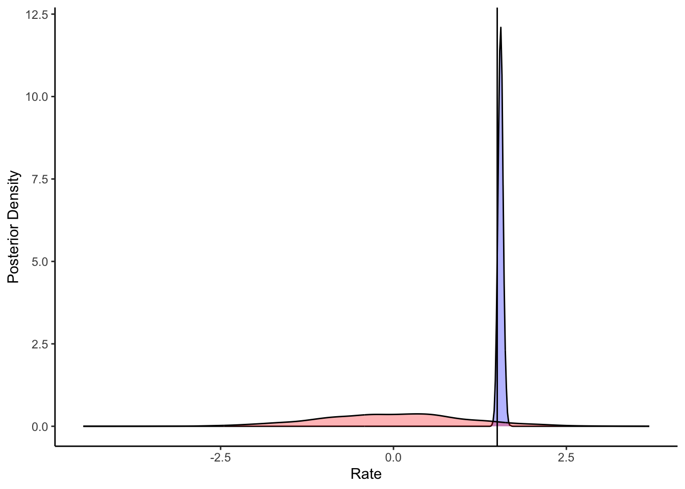
ggplot(draws_df) +
  geom_density(aes(`tau[1]`), fill = "blue", alpha = 0.3) +
  geom_density(aes(`winSD_prior`), fill = "red", alpha = 0.3) +
  geom_vline(xintercept = d$betaWinSD[1]) +
  xlab("Rate") +
  ylab("Posterior Density") +
  theme_classic()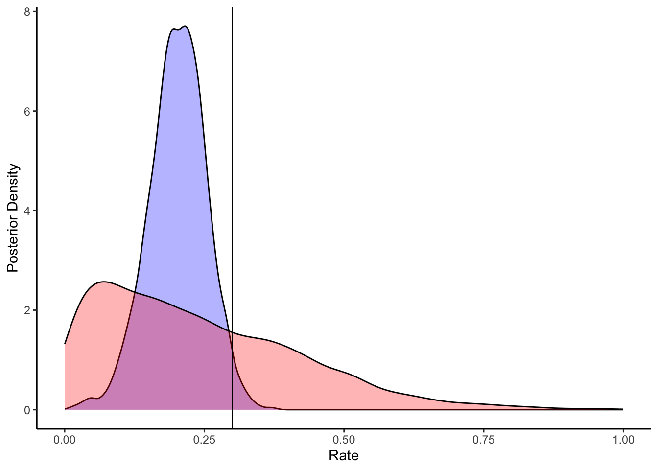
ggplot(draws_df) +
  geom_density(aes(loseM), fill = "blue", alpha = 0.3) +
  geom_density(aes(loseM_prior), fill = "red", alpha = 0.3) +
  geom_vline(xintercept = d$betaLoseM[1]) +
  xlab("Rate") +
  ylab("Posterior Density") +
  theme_classic()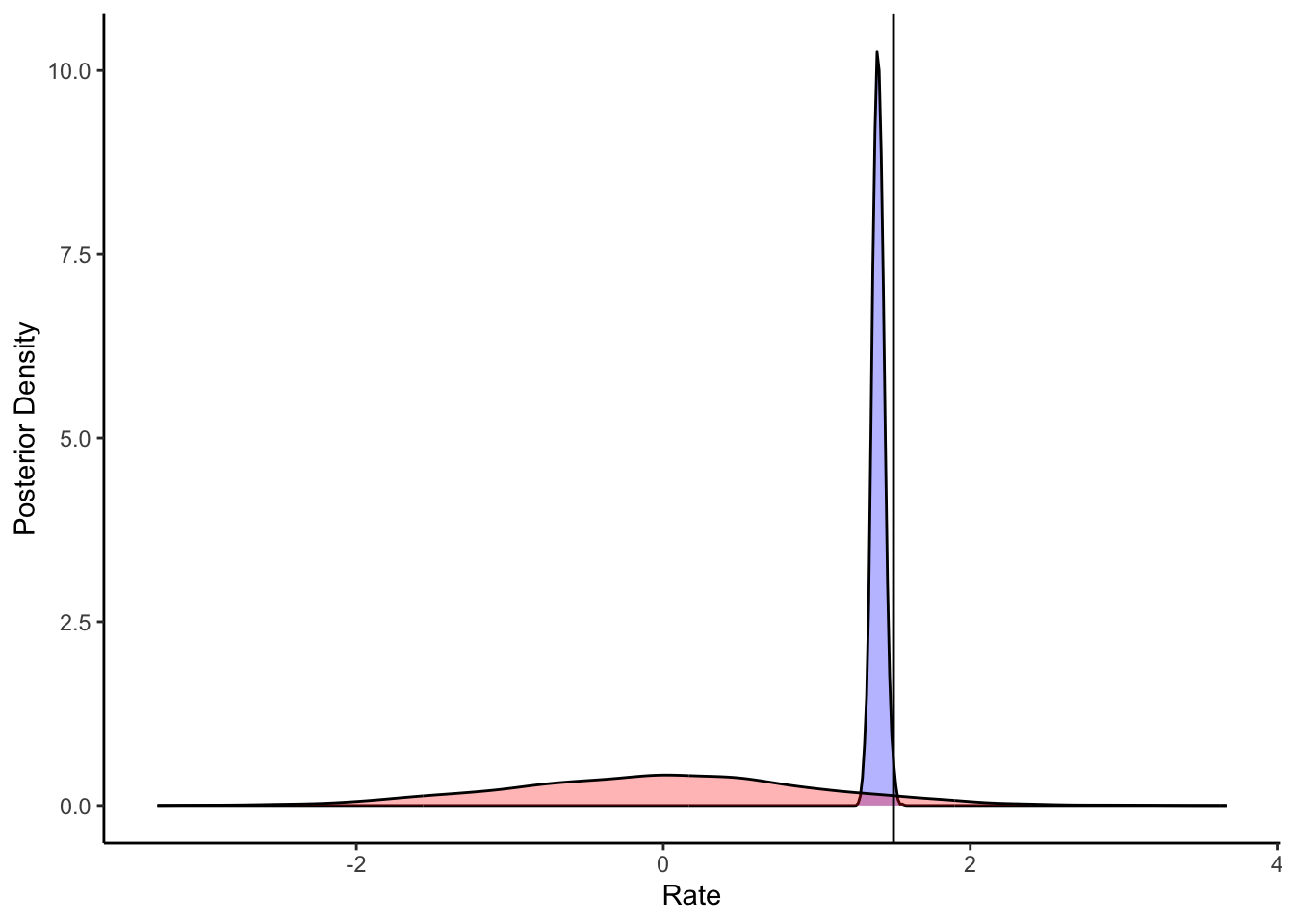
ggplot(draws_df) +
  geom_density(aes(`tau[2]`), fill = "blue", alpha = 0.3) +
  geom_density(aes(`loseSD_prior`), fill = "red", alpha = 0.3) +
  geom_vline(xintercept = d$betaLoseSD[1]) +
  xlab("Rate") +
  ylab("Posterior Density") +
  theme_classic()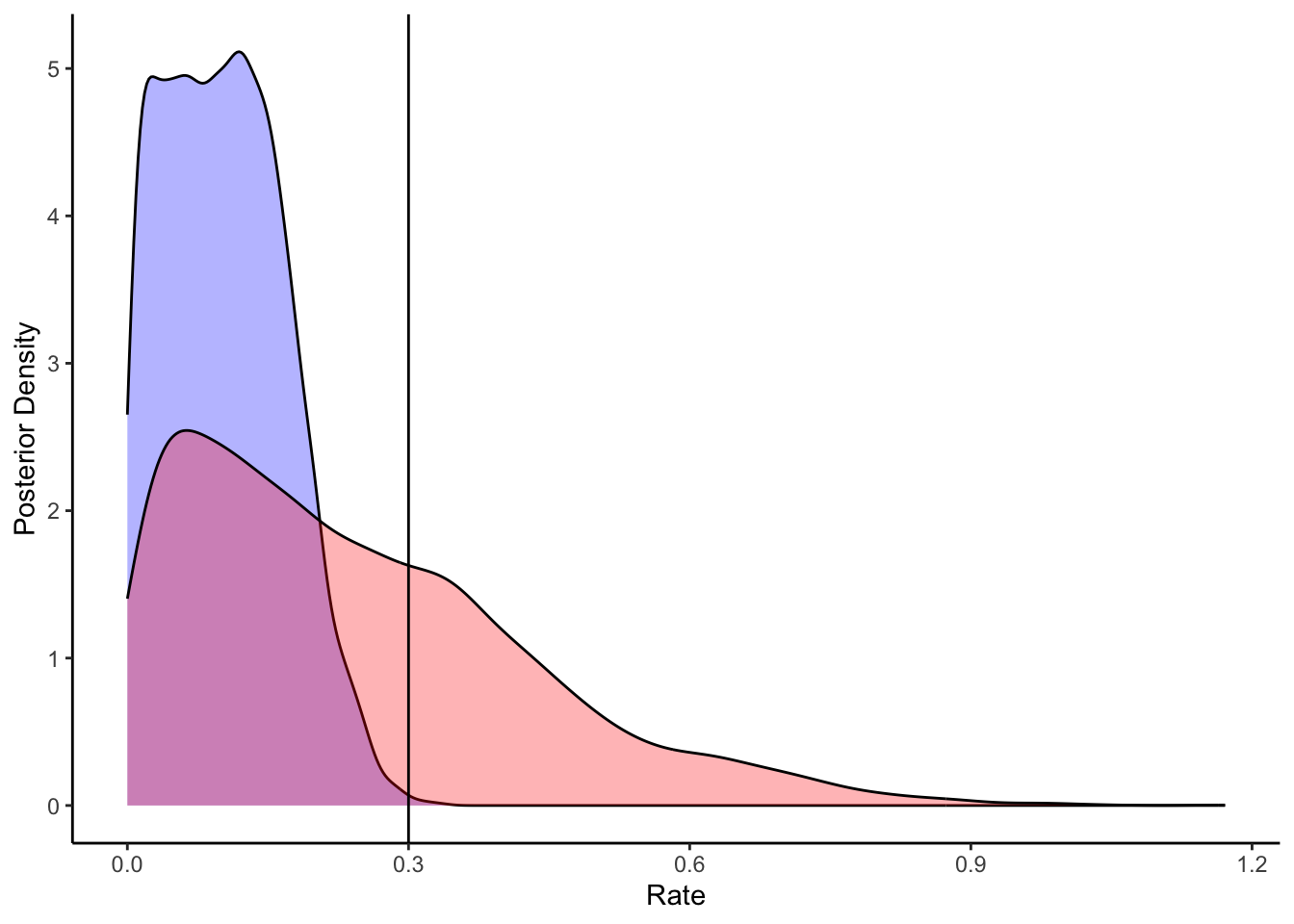
[MISSING: Model comparison with biased] [MISSING: Mixture model with biased]